Chapter 01: Getting Started

This notebook introduces the vangja time series forecasting package using the classic Air Passengers dataset (similar to how Facebook Prophet tutorials begin).

In This Notebook

We cover the fundamental concepts of vangja:

1. Loading data using vangja’s built-in dataset functions

2. Building models by composing trend and seasonality components

3. Additive vs multiplicative models and when to use each

4. Evaluating forecasts with standard metrics

Setup and Imports

import warnings

warnings.filterwarnings("ignore")

import matplotlib.pyplot as plt
import numpy as np
import pandas as pd

from vangja import FourierSeasonality, LinearTrend
from vangja.datasets import load_air_passengers
from vangja.utils import metrics

# Set random seed for reproducibility
np.random.seed(42)

print("Imports successful!")

Imports successful!

---

1. Load Air Passengers Dataset

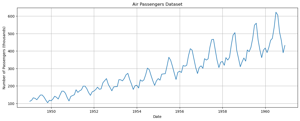
The Air Passengers dataset is a classic time series dataset containing monthly totals of international airline passengers from 1949 to 1960.

Vangja provides convenience functions in vangja.datasets to load common datasets in the expected format (columns: ds for datetime, y for target values).

# Load Air Passengers dataset using vangja.datasets
air_passengers = load_air_passengers()

print(f"Dataset shape: {air_passengers.shape}")
print(f"Date range: {air_passengers['ds'].min()} to {air_passengers['ds'].max()}")
air_passengers.head()

Dataset shape: (144, 2)
Date range: 1949-01-01 00:00:00 to 1960-12-01 00:00:00

	ds	y
0	1949-01-01	112
1	1949-02-01	118
2	1949-03-01	132
3	1949-04-01	129
4	1949-05-01	121

# Visualize the data
plt.figure(figsize=(14, 5))
plt.plot(air_passengers["ds"], air_passengers["y"])
plt.title("Air Passengers Dataset")
plt.xlabel("Date")
plt.ylabel("Number of Passengers (thousands)")
plt.grid(True)
plt.show()

---

2. Train/Test Split

We hold out the last 12 months of data as a test set. This lets us evaluate how well the model extrapolates beyond the training period.

# Split data: use last 12 months for testing
train = air_passengers[:-12].copy()
test = air_passengers[-12:].copy()

print(
    f"Training set: {train['ds'].min()} to {train['ds'].max()} ({len(train)} samples)"
)
print(f"Test set: {test['ds'].min()} to {test['ds'].max()} ({len(test)} samples)")

Training set: 1949-01-01 00:00:00 to 1959-12-01 00:00:00 (132 samples)
Test set: 1960-01-01 00:00:00 to 1960-12-01 00:00:00 (12 samples)

---

3. Model Air Passengers like Facebook Prophet

Facebook Prophet models time series as a sum of interpretable components:

• Trend component (piecewise linear or logistic growth)

• Seasonality component (Fourier series)

• Holiday effects (optional)

For the Air Passengers dataset, we observe:

• A clear upward trend

• Strong yearly seasonality

• Multiplicative seasonality (the seasonal amplitude increases with the level)

Vangja uses operator overloading to compose models from these building blocks:

Operator	Meaning	Formula
+	Additive	\(y = \text{left} + \text{right}\)
**	Multiplicative (Prophet-style)	\(y = \text{left} \cdot (1 + \text{right})\)
*	Simple multiplicative	\(y = \text{left} \cdot \text{right}\)

3.1 Additive Model

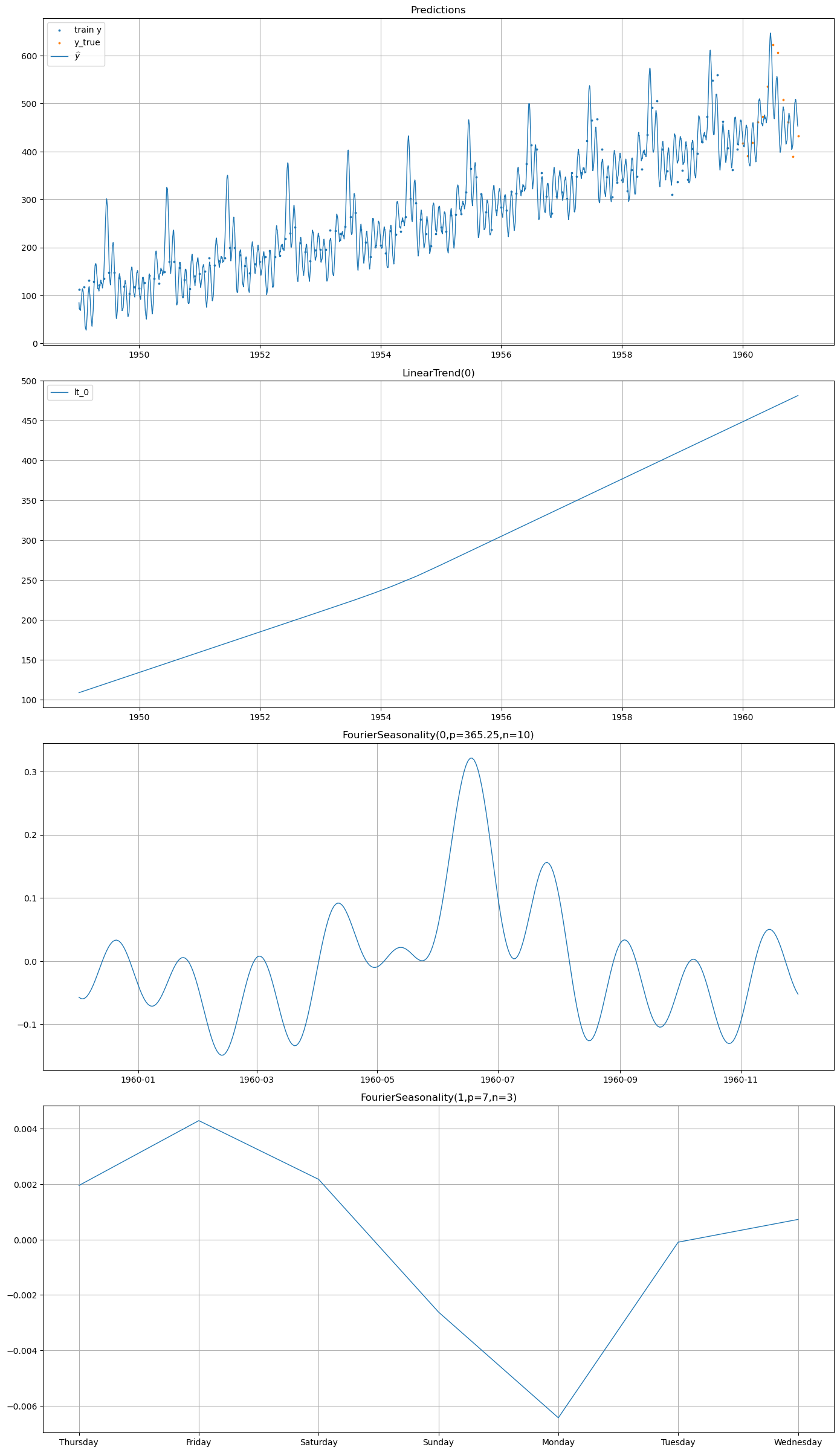
An additive model assumes the final value is the sum of its components: \(y(t) = g(t) + s(t) + \epsilon\). Here, LinearTrend() captures the upward growth and FourierSeasonality() captures repeating patterns at yearly and weekly frequencies.

# Define an additive model: Trend + Yearly Seasonality + Weekly Seasonality
model_additive = (
    LinearTrend()
    + FourierSeasonality(period=365.25, series_order=10)
    + FourierSeasonality(period=7, series_order=3)
)

print(f"Model: {model_additive}")

Model: LT(n=25,r=0.8,tm=None) + FS(p=365.25,n=10,tm=None) + FS(p=7,n=3,tm=None)

# Fit the additive model
model_additive.fit(train)
print("Additive model fitted!")

WARNING:2026-02-26 20:40:24,367:jax._src.xla_bridge:876: An NVIDIA GPU may be present on this machine, but a CUDA-enabled jaxlib is not installed. Falling back to cpu.

Additive model fitted!

# Predict
future_additive = model_additive.predict(horizon=365, freq="D")
print(f"Predictions shape: {future_additive.shape}")
future_additive.head()

Predictions shape: (4352, 6)

	ds	t	lt_0_0	fs_0_0	fs_1_0	yhat_0
0	1949-01-01	0.000000	108.462884	-0.044380	0.002170	84.867545
1	1949-01-02	0.000251	108.532605	-0.051900	-0.002614	78.058796
2	1949-01-03	0.000502	108.602326	-0.058430	-0.006427	72.347272
3	1949-01-04	0.000753	108.672047	-0.063777	-0.000094	72.968074
4	1949-01-05	0.001004	108.741768	-0.067789	0.000725	71.252909

# Plot results
plt.figure(figsize=(14, 5))
plt.plot(train["ds"], train["y"], "b.", label="Training data", markersize=3)
plt.plot(test["ds"], test["y"], "g.", label="Test data", markersize=3)
plt.plot(
    future_additive["ds"],
    future_additive["yhat_0"],
    "r-",
    label="Prediction",
    linewidth=1,
)
plt.title("Additive Model: Air Passengers")
plt.xlabel("Date")
plt.ylabel("Number of Passengers")
plt.legend()
plt.grid(True)
plt.show()

model_additive.plot(future_additive, y_true=test)
plt.tight_layout()
plt.show()

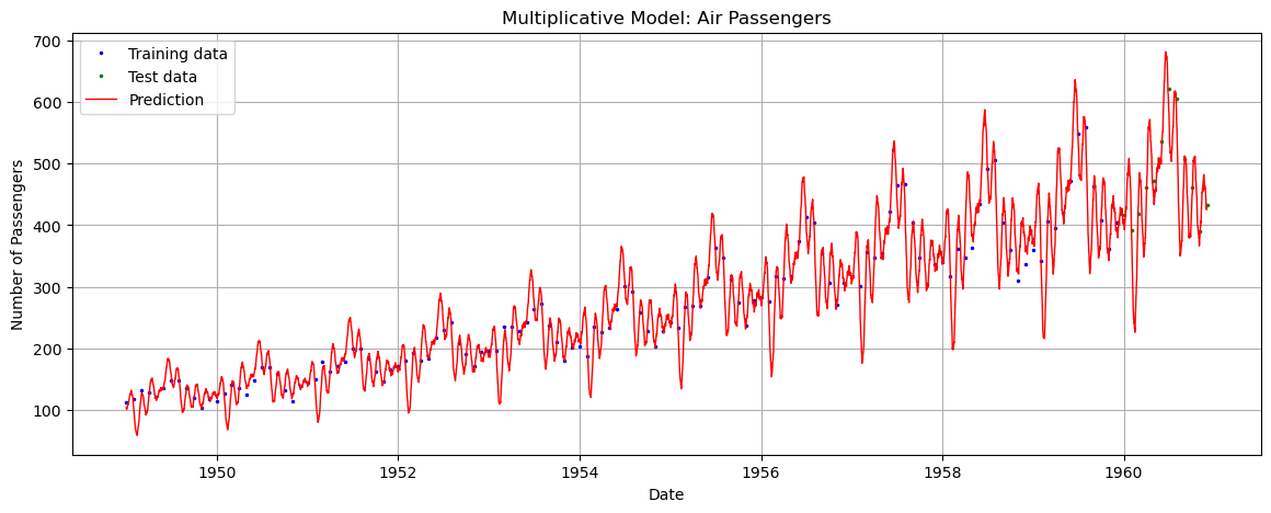
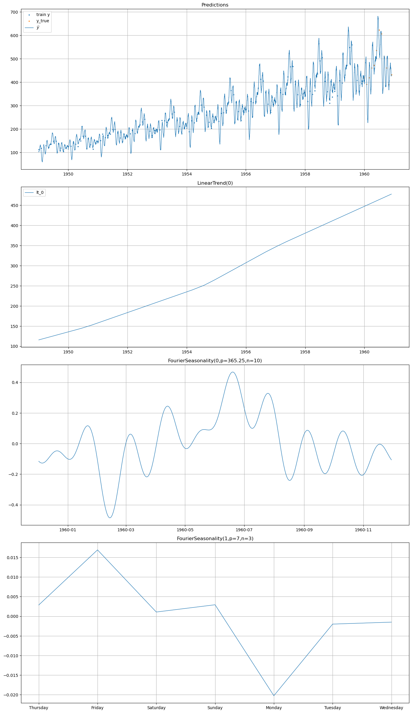
3.2 Multiplicative Model

The Air Passengers data shows multiplicative seasonality — the variance of the seasonal fluctuations increases with the trend level. A multiplicative model captures this via: \(y(t) = g(t) \cdot (1 + s(t)) + \epsilon\)

In vangja, the ** operator creates this multiplicative relationship.

# Define a multiplicative model
model_mult = LinearTrend() ** (
    FourierSeasonality(period=365.25, series_order=10)
    + FourierSeasonality(period=7, series_order=3)
)

print(f"Model: {model_mult}")

Model: LT(n=25,r=0.8,tm=None) * (1 + FS(p=365.25,n=10,tm=None) + FS(p=7,n=3,tm=None))

# Fit the multiplicative model
model_mult.fit(train)
print("Multiplicative model fitted!")

Multiplicative model fitted!

We plot the results to show how the multiplicative seasonality better captures the increase of variance with the trend.

# Predict
future_mult = model_mult.predict(horizon=365, freq="D")

# Plot results
plt.figure(figsize=(14, 5))
plt.plot(train["ds"], train["y"], "b.", label="Training data", markersize=3)
plt.plot(test["ds"], test["y"], "g.", label="Test data", markersize=3)
plt.plot(
    future_mult["ds"], future_mult["yhat_0"], "r-", label="Prediction", linewidth=1
)
plt.title("Multiplicative Model: Air Passengers")
plt.xlabel("Date")
plt.ylabel("Number of Passengers")
plt.legend()
plt.grid(True)
plt.show()

model_mult.plot(future_mult, y_true=test)
plt.tight_layout()
plt.show()

Metrics Comparison

We compare standard forecasting metrics between the additive and multiplicative models. Lower values are better for all metrics: MSE (mean squared error), RMSE (root mean squared error), MAE (mean absolute error), and MAPE (mean absolute percentage error).

metrics_additive = metrics(test, future_additive, "complete")
print("Additive Model Metrics:")
display(metrics_additive)

Additive Model Metrics:

	mse	rmse	mae	mape
series	1988.497349	44.592571	34.349423	0.067574

metrics_mult = metrics(test, future_mult, "complete")
print("Multiplicative Model Metrics:")
display(metrics_mult)

Multiplicative Model Metrics:

	mse	rmse	mae	mape
series	629.010786	25.080087	21.254398	0.04267

---

Summary

In this chapter, we introduced the core modeling pattern of vangja using the Air Passengers dataset:

1. Additive model (+): Combines trend and seasonality as \(y = g(t) + s(t) + \epsilon\). Works well when the seasonal amplitude is roughly constant over time.

2. Multiplicative model (**): Combines trend and seasonality as \(y = g(t) \cdot (1 + s(t)) + \epsilon\). Better suited when the seasonal amplitude grows proportionally with the level — as we see in the Air Passengers data.

The multiplicative model generally produces better forecasts for this dataset because the variance of the seasonal fluctuations increases with the number of passengers over the years.

What’s Next

In Chapter 02, we explore the different Bayesian inference algorithms available in vangja — MAP, Variational Inference, and MCMC — and compare their speed, accuracy, and uncertainty quantification capabilities.