Chapter 04: Multi-Series Fitting Caveats#
In Chapter 03, we demonstrated how vangja’s simultaneous fitting provides equivalent results to sequential fitting when series share the same time range. But what happens when series have different date ranges?
This notebook explores the caveats and gotchas that arise when fitting series with non-overlapping time ranges, using real-world datasets as examples.
Key takeaways:
Changepoints are distributed across the combined time range, diluting coverage per series
Series with different date ranges may get fewer changepoints than expected
Use
filter_predictions_by_series()to extract predictions for each series’ relevant date rangeConsider fitting series with similar date ranges together, or increasing
n_changepointsto compensate
Setup and Imports#
[1]:
import warnings

warnings.filterwarnings("ignore")
[2]:
import time

import matplotlib.pyplot as plt
import numpy as np
import pandas as pd

from vangja import FourierSeasonality, LinearTrend
from vangja.datasets import load_air_passengers, load_peyton_manning
from vangja.utils import filter_predictions_by_series, metrics

print("Imports successful!")
Imports successful!
Load Real-World Datasets#
We’ll use two classic datasets with very different date ranges:
Air Passengers: Monthly airline passengers, 1949-1960 (more than 40 years before the Peyton Manning Wikipedia Views dataset!)
Peyton Manning Wikipedia Views: Daily page views, 2007-2016
Both datasets are available in vangja.datasets.
[3]:
# Load datasets from vangja.datasets
air_passengers = load_air_passengers()
air_passengers["series"] = "air_passengers"

peyton_manning = load_peyton_manning()
peyton_manning["series"] = "peyton_manning"

print(
    f"Air Passengers: {air_passengers['ds'].min().date()} to {air_passengers['ds'].max().date()} ({len(air_passengers)} samples, monthly)"
)
print(
    f"Peyton Manning: {peyton_manning['ds'].min().date()} to {peyton_manning['ds'].max().date()} ({len(peyton_manning)} samples, daily)"
)
Air Passengers: 1949-01-01 to 1960-12-01 (144 samples, monthly)
Peyton Manning: 2007-12-10 to 2016-01-20 (2905 samples, daily)
[4]:
# Visualize the date ranges
fig, axes = plt.subplots(1, 2, figsize=(14, 4))

axes[0].plot(air_passengers["ds"], air_passengers["y"], "b-")
axes[0].set_title("Air Passengers (1949-1960)")
axes[0].set_xlabel("Date")
axes[0].set_ylabel("Passengers")
axes[0].grid(True, alpha=0.3)

axes[1].plot(peyton_manning["ds"], peyton_manning["y"], "r-", linewidth=0.5)
axes[1].set_title("Peyton Manning Wikipedia Views (2007-2016)")
axes[1].set_xlabel("Date")
axes[1].set_ylabel("Log Views")
axes[1].grid(True, alpha=0.3)

plt.tight_layout()
plt.show()

print(
    f"\nTime gap between series: {(peyton_manning['ds'].min() - air_passengers['ds'].max()).days} days (~47 years!)"
)
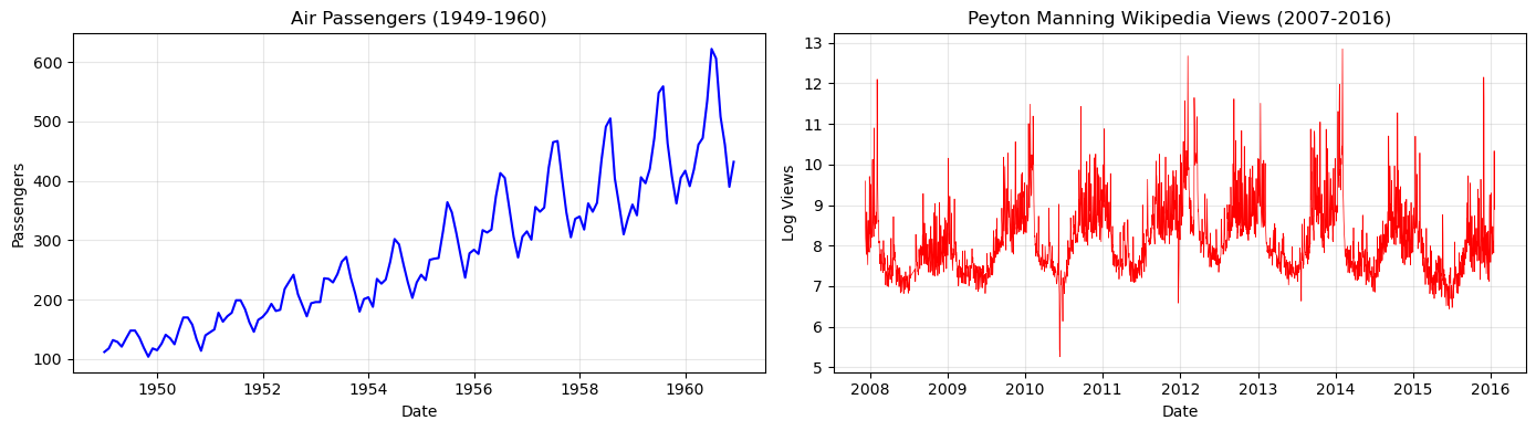
Time gap between series: 17175 days (~47 years!)
Understanding the Caveat: Changepoint Distribution#
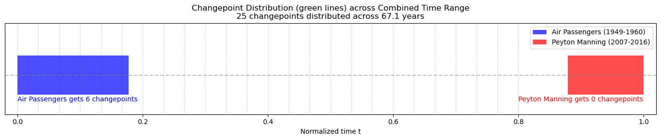
The problem: When fitting multiple series simultaneously, vangja normalizes time to t = [0, 1] across the entire combined time range. This has two important consequences:
Time compression: Each series occupies only a small portion of the normalized time range
Changepoint dilution: The
n_changepointsare distributed across the full range, so each series may get very few changepoints in its actual date range
Let’s visualize this:
[5]:
# Calculate normalized time ranges
combined_min = min(air_passengers["ds"].min(), peyton_manning["ds"].min())
combined_max = max(air_passengers["ds"].max(), peyton_manning["ds"].max())
combined_range_days = (combined_max - combined_min).days

# Air Passengers normalized range
ap_t_min = (air_passengers["ds"].min() - combined_min).days / combined_range_days
ap_t_max = (air_passengers["ds"].max() - combined_min).days / combined_range_days

# Peyton Manning normalized range
pm_t_min = (peyton_manning["ds"].min() - combined_min).days / combined_range_days
pm_t_max = (peyton_manning["ds"].max() - combined_min).days / combined_range_days

print(
    f"Combined time range: {combined_min.date()} to {combined_max.date()} ({combined_range_days} days, ~{combined_range_days/365:.1f} years)"
)
print("\nNormalized t = [0, 1] distribution:")
print(
    f"  Air Passengers: t = [{ap_t_min:.3f}, {ap_t_max:.3f}] (only {(ap_t_max - ap_t_min)*100:.1f}% of range)"
)
print(
    f"  Peyton Manning: t = [{pm_t_min:.3f}, {pm_t_max:.3f}] (only {(pm_t_max - pm_t_min)*100:.1f}% of range)"
)

# Estimate changepoints per series with n_changepoints=25
n_changepoints = 25
ap_expected_cp = (
    n_changepoints * (ap_t_max - ap_t_min) * 0.8
)  # 80% of data for changepoints
pm_expected_cp = n_changepoints * (pm_t_max - pm_t_min) * 0.8

print(f"\nWith n_changepoints={n_changepoints} distributed across combined range:")
print(
    f"  Air Passengers: ~{ap_expected_cp:.1f} changepoints expected (vs 25 if fit separately)"
)
print(
    f"  Peyton Manning: ~{pm_expected_cp:.1f} changepoints expected (vs 25 if fit separately)"
)
Combined time range: 1949-01-01 to 2016-01-20 (24490 days, ~67.1 years)

Normalized t = [0, 1] distribution:
  Air Passengers: t = [0.000, 0.178] (only 17.8% of range)
  Peyton Manning: t = [0.879, 1.000] (only 12.1% of range)

With n_changepoints=25 distributed across combined range:
  Air Passengers: ~3.6 changepoints expected (vs 25 if fit separately)
  Peyton Manning: ~2.4 changepoints expected (vs 25 if fit separately)
[6]:
# Visualize the time normalization issue
fig, ax = plt.subplots(figsize=(14, 3))

# Draw the normalized time range [0, 1]
ax.axhline(y=0, color="gray", linestyle="--", alpha=0.5)

# Air Passengers range
ax.barh(
    0,
    ap_t_max - ap_t_min,
    left=ap_t_min,
    height=0.3,
    color="blue",
    alpha=0.7,
    label="Air Passengers (1949-1960)",
)

# Peyton Manning range
ax.barh(
    0,
    pm_t_max - pm_t_min,
    left=pm_t_min,
    height=0.3,
    color="red",
    alpha=0.7,
    label="Peyton Manning (2007-2016)",
)

# Changepoints (evenly distributed)
changepoint_positions = np.linspace(0, 0.8, n_changepoints)  # Default is 80% of range
for cp in changepoint_positions:
    ax.axvline(x=cp, color="green", linestyle=":", alpha=0.4, linewidth=0.8)

ax.set_xlim(-0.02, 1.02)
ax.set_ylim(-0.3, 0.4)
ax.set_xlabel("Normalized time t")
ax.set_yticks([])
ax.set_title(
    f"Changepoint Distribution (green lines) across Combined Time Range\n{n_changepoints} changepoints distributed across {combined_range_days/365:.1f} years"
)
ax.legend(loc="upper right")

# Count changepoints in each series range
cp_in_ap = sum(1 for cp in changepoint_positions if ap_t_min <= cp <= ap_t_max)
cp_in_pm = sum(1 for cp in changepoint_positions if pm_t_min <= cp <= pm_t_max)
ax.text(
    0,
    -0.2,
    f"Air Passengers gets {cp_in_ap} changepoints",
    fontsize=10,
    color="blue",
)
ax.text(
    0.8, -0.2, f"Peyton Manning gets {cp_in_pm} changepoints", fontsize=10, color="red"
)

plt.tight_layout()
plt.show()
Demonstrating the Impact#
Let’s fit both series using:
Sequential fitting: Each series fit independently (baseline)
Simultaneous fitting: Both series fit together
[7]:
# Prepare train/test splits
# Air Passengers: hold out last 24 months (monthly data)
train_passengers = air_passengers[:-24].copy()
test_passengers = air_passengers[-24:].copy()

# Peyton Manning: hold out last 365 days (daily data)
train_peyton = peyton_manning[:-365].copy()
test_peyton = peyton_manning[-365:].copy()

# Combined training data
train_combined = pd.concat([train_passengers, train_peyton], ignore_index=True)

print(
    f"Air Passengers training: {len(train_passengers)} months, test: {len(test_passengers)} months"
)
print(
    f"Peyton Manning training: {len(train_peyton)} days, test: {len(test_peyton)} days"
)
Air Passengers training: 120 months, test: 24 months
Peyton Manning training: 2540 days, test: 365 days
Sequential Fitting (Baseline)#
[8]:
# Fit Air Passengers sequentially
model_passengers_seq = (
    LinearTrend()
    + FourierSeasonality(period=365.25, series_order=10)
    + FourierSeasonality(period=12, series_order=5)
    + FourierSeasonality(
        period=7, series_order=3
    )  # Add weekly seasonality (even if not expected)
)

start_time = time.time()
model_passengers_seq.fit(train_passengers, method="mapx")
time_passengers_seq = time.time() - start_time

print(f"Air Passengers sequential fit: {time_passengers_seq:.2f}s")
WARNING:2026-02-27 00:14:32,333:jax._src.xla_bridge:876: An NVIDIA GPU may be present on this machine, but a CUDA-enabled jaxlib is not installed. Falling back to cpu.
Air Passengers sequential fit: 3.91s
[9]:
# Fit Peyton Manning sequentially
model_peyton_seq = (
    LinearTrend()
    + FourierSeasonality(period=365.25, series_order=10)
    + FourierSeasonality(period=12, series_order=5)
    + FourierSeasonality(period=7, series_order=3)
)

start_time = time.time()
model_peyton_seq.fit(train_peyton, method="mapx")
time_peyton_seq = time.time() - start_time

print(f"Peyton Manning sequential fit: {time_peyton_seq:.2f}s")
print(f"Total sequential time: {time_passengers_seq + time_peyton_seq:.2f}s")
Peyton Manning sequential fit: 2.98s
Total sequential time: 6.90s
[10]:
# Sequential predictions and metrics
future_passengers_seq = model_passengers_seq.predict(horizon=730, freq="D")  # Monthly
future_peyton_seq = model_peyton_seq.predict(horizon=365, freq="D")  # Daily

metrics_passengers_seq = metrics(test_passengers, future_passengers_seq, "complete")
metrics_peyton_seq = metrics(test_peyton, future_peyton_seq, "complete")

print("Sequential Fitting Metrics:")
print("Air Passengers:")
display(metrics_passengers_seq)
print("Peyton Manning:")
display(metrics_peyton_seq)
Sequential Fitting Metrics:
Air Passengers:
| mse | rmse | mae | mape | |
|---|---|---|---|---|
| air_passengers | 2026.910512 | 45.021223 | 34.40509 | 0.071895 |
Peyton Manning:
| mse | rmse | mae | mape | |
|---|---|---|---|---|
| peyton_manning | 0.302963 | 0.550421 | 0.43198 | 0.055724 |
Simultaneous Fitting#
[11]:
# Create model for simultaneous fitting
model_combined = (
    LinearTrend(pool_type="individual", delta_pool_type="individual")
    + FourierSeasonality(period=365.25, series_order=10, pool_type="individual")
    + FourierSeasonality(period=12, series_order=5, pool_type="individual")
    + FourierSeasonality(period=7, series_order=3, pool_type="individual")
)

start_time = time.time()
model_combined.fit(train_combined, method="mapx", scale_mode="individual")
time_combined = time.time() - start_time

print(f"Simultaneous fitting time: {time_combined:.2f}s")
print(f"Group mapping: {model_combined.groups_}")
Simultaneous fitting time: 3.26s
Group mapping: {0: 'air_passengers', 1: 'peyton_manning'}
[12]:
# Generate predictions
# The prediction spans the entire combined time range plus horizon!
future_combined = model_combined.predict(horizon=730, freq="D")

print(
    f"Combined prediction date range: {future_combined['ds'].min().date()} to {future_combined['ds'].max().date()}"
)
print(f"That's {len(future_combined)} rows!")
print(
    f"\nPrediction columns: {[col for col in future_combined.columns if 'yhat' in col]}"
)
Combined prediction date range: 1949-01-01 to 2017-01-17
That's 24854 rows!

Prediction columns: ['yhat_0', 'yhat_1']
Using filter_predictions_by_series()#
When fitting series with different date ranges, predictions span the entire combined time range. Use filter_predictions_by_series() to get predictions for each series’ relevant date range:
[13]:
# Get group codes
group_mapping = model_combined.groups_
passengers_group = [k for k, v in group_mapping.items() if v == "air_passengers"][0]
peyton_group = [k for k, v in group_mapping.items() if v == "peyton_manning"][0]

print(f"Air Passengers group: {passengers_group}")
print(f"Peyton Manning group: {peyton_group}")
Air Passengers group: 0
Peyton Manning group: 1
[14]:
# Filter predictions for Air Passengers
future_passengers_combined = filter_predictions_by_series(
    future=future_combined,
    series_data=train_passengers,
    yhat_col=f"yhat_{passengers_group}",
    horizon=730,
)

# Filter predictions for Peyton Manning
future_peyton_combined = filter_predictions_by_series(
    future=future_combined,
    series_data=train_peyton,
    yhat_col=f"yhat_{peyton_group}",
    horizon=365,
)

print(f"Filtered Air Passengers predictions: {len(future_passengers_combined)} rows")
print(
    f"  Date range: {future_passengers_combined['ds'].min().date()} to {future_passengers_combined['ds'].max().date()}"
)
print(f"\nFiltered Peyton Manning predictions: {len(future_peyton_combined)} rows")
print(
    f"  Date range: {future_peyton_combined['ds'].min().date()} to {future_peyton_combined['ds'].max().date()}"
)
Filtered Air Passengers predictions: 4352 rows
  Date range: 1949-01-01 to 1960-11-30

Filtered Peyton Manning predictions: 2962 rows
  Date range: 2007-12-10 to 2016-01-18
[15]:
# Calculate metrics using filtered predictions
# Note: Need to rename column to yhat_0 for metrics() function
future_passengers_for_metrics = future_passengers_combined.rename(
    columns={f"yhat_{passengers_group}": "yhat_0"}
)
future_peyton_for_metrics = future_peyton_combined.rename(
    columns={f"yhat_{peyton_group}": "yhat_0"}
)

metrics_passengers_combined = metrics(
    test_passengers, future_passengers_for_metrics, "complete"
)
metrics_peyton_combined = metrics(test_peyton, future_peyton_for_metrics, "complete")

print("Simultaneous Fitting Metrics:")
print("\nAir Passengers:")
display(metrics_passengers_combined)
print("\nPeyton Manning:")
display(metrics_peyton_combined)
Simultaneous Fitting Metrics:

Air Passengers:
| mse | rmse | mae | mape | |
|---|---|---|---|---|
| air_passengers | 2625.193777 | 51.236645 | 36.072534 | 0.071156 |
Peyton Manning:
| mse | rmse | mae | mape | |
|---|---|---|---|---|
| peyton_manning | 0.893486 | 0.945244 | 0.875799 | 0.114976 |
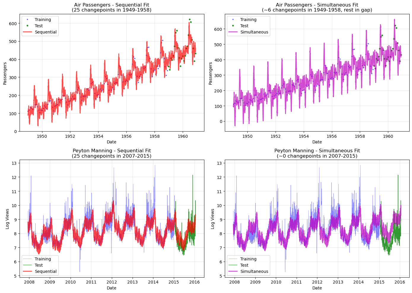
Comparison: Sequential vs Simultaneous#
Let’s compare the metrics side-by-side to see the impact of changepoint dilution:
[16]:
# Create comparison table
comparison_data = []

for series_name, seq_metrics, sim_metrics in [
    ("Air Passengers", metrics_passengers_seq, metrics_passengers_combined),
    ("Peyton Manning", metrics_peyton_seq, metrics_peyton_combined),
]:
    comparison_data.append(
        {
            "Series": series_name,
            "Approach": "Sequential",
            "RMSE": seq_metrics["rmse"].values[0],
            "MAE": seq_metrics["mae"].values[0],
            "MAPE": seq_metrics["mape"].values[0],
        }
    )
    comparison_data.append(
        {
            "Series": series_name,
            "Approach": "Simultaneous",
            "RMSE": sim_metrics["rmse"].values[0],
            "MAE": sim_metrics["mae"].values[0],
            "MAPE": sim_metrics["mape"].values[0],
        }
    )

metrics_comparison = pd.DataFrame(comparison_data)
print("Metrics Comparison:")
display(metrics_comparison)
Metrics Comparison:
| Series | Approach | RMSE | MAE | MAPE | |
|---|---|---|---|---|---|
| 0 | Air Passengers | Sequential | 45.021223 | 34.405090 | 0.071895 |
| 1 | Air Passengers | Simultaneous | 51.236645 | 36.072534 | 0.071156 |
| 2 | Peyton Manning | Sequential | 0.550421 | 0.431980 | 0.055724 |
| 3 | Peyton Manning | Simultaneous | 0.945244 | 0.875799 | 0.114976 |
[17]:
# Visual comparison
fig, axes = plt.subplots(2, 2, figsize=(14, 10))

# Air Passengers
ax = axes[0, 0]
ax.plot(
    train_passengers["ds"],
    train_passengers["y"],
    "b.",
    markersize=4,
    alpha=0.5,
    label="Training",
)
ax.plot(
    test_passengers["ds"],
    test_passengers["y"],
    "g.",
    markersize=6,
    alpha=0.8,
    label="Test",
)
ax.plot(
    future_passengers_seq["ds"],
    future_passengers_seq["yhat_0"],
    "r-",
    linewidth=2,
    alpha=0.7,
    label="Sequential",
)
ax.set_title("Air Passengers - Sequential Fit\n(25 changepoints in 1949-1958)")
ax.set_xlabel("Date")
ax.set_ylabel("Passengers")
ax.legend()
ax.grid(True, alpha=0.3)

ax = axes[0, 1]
ax.plot(
    train_passengers["ds"],
    train_passengers["y"],
    "b.",
    markersize=4,
    alpha=0.5,
    label="Training",
)
ax.plot(
    test_passengers["ds"],
    test_passengers["y"],
    "g.",
    markersize=6,
    alpha=0.8,
    label="Test",
)
ax.plot(
    future_passengers_combined["ds"],
    future_passengers_combined[f"yhat_{passengers_group}"],
    "m-",
    linewidth=2,
    alpha=0.7,
    label="Simultaneous",
)
ax.set_title(
    f"Air Passengers - Simultaneous Fit\n(~{cp_in_ap} changepoints in 1949-1958, rest in gap)"
)
ax.set_xlabel("Date")
ax.set_ylabel("Passengers")
ax.legend()
ax.grid(True, alpha=0.3)

# Peyton Manning
ax = axes[1, 0]
ax.plot(
    train_peyton["ds"],
    train_peyton["y"],
    "b-",
    linewidth=0.5,
    alpha=0.5,
    label="Training",
)
ax.plot(test_peyton["ds"], test_peyton["y"], "g-", linewidth=1, alpha=0.8, label="Test")
ax.plot(
    future_peyton_seq["ds"],
    future_peyton_seq["yhat_0"],
    "r-",
    linewidth=2,
    alpha=0.7,
    label="Sequential",
)
ax.set_title("Peyton Manning - Sequential Fit\n(25 changepoints in 2007-2015)")
ax.set_xlabel("Date")
ax.set_ylabel("Log Views")
ax.legend()
ax.grid(True, alpha=0.3)

ax = axes[1, 1]
ax.plot(
    train_peyton["ds"],
    train_peyton["y"],
    "b-",
    linewidth=0.5,
    alpha=0.5,
    label="Training",
)
ax.plot(test_peyton["ds"], test_peyton["y"], "g-", linewidth=1, alpha=0.8, label="Test")
ax.plot(
    future_peyton_combined["ds"],
    future_peyton_combined["yhat_0"],
    "m-",
    linewidth=2,
    alpha=0.7,
    label="Simultaneous",
)
ax.set_title(
    f"Peyton Manning - Simultaneous Fit\n(~{cp_in_pm} changepoints in 2007-2015)"
)
ax.set_xlabel("Date")
ax.set_ylabel("Log Views")
ax.legend()
ax.grid(True, alpha=0.3)

plt.tight_layout()
plt.show()
Summary and Recommendations#
Key Findings#
Different results are expected: When series have very different date ranges, simultaneous and sequential fitting will produce different results due to changepoint distribution.
Changepoint dilution: With a ~60-year combined time range but each series only covering ~10 years, each series only gets a fraction of the specified changepoints.
This is not a bug: This is expected behavior. Changepoints are placed in normalized time
t = [0, 1], which spans the entire combined date range.
Recommendations#
Scenario |
Recommendation |
|---|---|
Series with same time range |
✅ Use simultaneous fitting (see Chapter 03) |
Series with overlapping time ranges |
✅ Simultaneous fitting works well |
Series with non-overlapping ranges |
⚠️ Consider sequential fitting |
Series with large time gaps |
❌ Fit separately for best results |
Workarounds#
If you must fit series with different date ranges simultaneously:
Increase ``n_changepoints``: Compensate for dilution by increasing the total number of changepoints
Group similar series: Fit series with similar date ranges together
Use hierarchical pooling: Consider
pool_type="partial"to share information across series while maintaining flexibilityFilter predictions: Use
filter_predictions_by_series()to get the correct date range for each series
What’s Next#
So far we have treated each series as independent (using pool_type="individual"). In Chapter 05, we introduce hierarchical Bayesian modeling with partial pooling — a powerful technique that lets related time series share statistical strength while preserving individual differences.