Chapter 03: Multi-Series Fitting#
This notebook demonstrates one of vangja’s key features: vectorized multi-series fitting. Unlike Facebook Prophet, which fits time series one at a time, vangja can fit multiple time series simultaneously using vectorized computations.
We’ll compare two approaches:
Sequential fitting (Prophet-style): Fit each time series independently, one after another
Simultaneous fitting (Vangja-style): Fit all time series at once with
pool_type="individual"
Both approaches produce equivalent results when series share the same time range, but the vectorized approach is significantly faster when you have many time series.
Note: For series with different date ranges, see Chapter 04 which covers important caveats.
Setup and Imports#
[1]:
import warnings

warnings.filterwarnings("ignore")
[2]:
import time

import matplotlib.pyplot as plt
import numpy as np
import pandas as pd

from vangja import FourierSeasonality, LinearTrend
from vangja.datasets import generate_multi_store_data
from vangja.utils import metrics

# Set random seed for reproducibility
np.random.seed(42)

print("Imports successful!")
Imports successful!
Generate Synthetic Multi-Store Data#
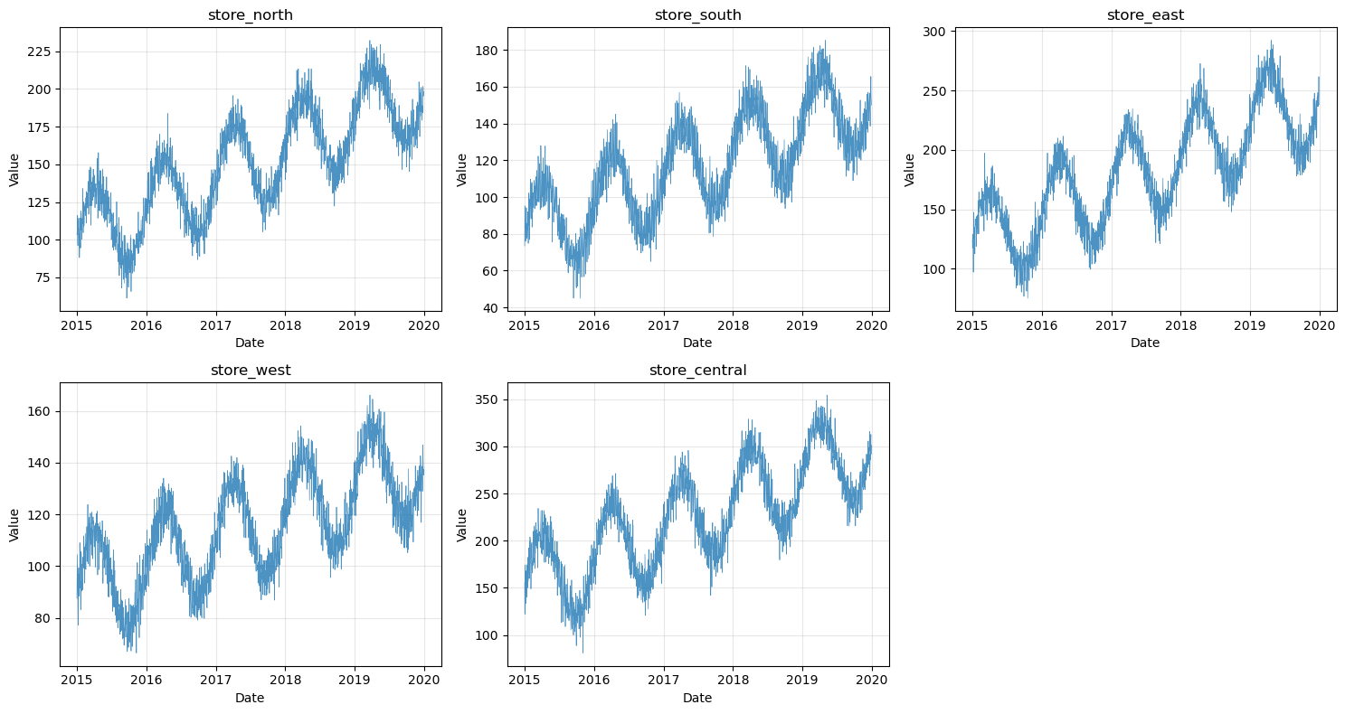
We’ll use 5 synthetic time series representing different stores, all sharing the same time range (2015-2020). This is the ideal scenario for simultaneous fitting.
Each series has:
A linear trend with different slopes
Yearly seasonality with different amplitudes
Weekly seasonality
Random noise
Vangja provides generate_multi_store_data() in vangja.datasets for this purpose.
[3]:
# Generate synthetic multi-store data
all_data, series_params = generate_multi_store_data(seed=42)

# Split into individual series for later use
all_series = [
    all_data[all_data["series"] == name].reset_index(drop=True)
    for name in all_data["series"].unique()
]

print(f"Date range: {all_data['ds'].min().date()} to {all_data['ds'].max().date()}")
print(f"Total days per series: {len(all_series[0])}")
print(f"Number of series: {len(all_series)}")
Date range: 2015-01-01 to 2019-12-31
Total days per series: 1826
Number of series: 5
[4]:
# Display series information
for params in series_params:
    series_df = all_data[all_data["series"] == params["name"]]
    print(
        f"{params['name']}: {len(series_df)} samples, y range: {series_df['y'].min():.1f} to {series_df['y'].max():.1f}"
    )

print(f"\nTotal combined data: {len(all_data)} samples")
store_north: 1826 samples, y range: 61.2 to 232.2
store_south: 1826 samples, y range: 45.0 to 185.2
store_east: 1826 samples, y range: 75.1 to 292.2
store_west: 1826 samples, y range: 66.5 to 166.1
store_central: 1826 samples, y range: 81.0 to 354.4

Total combined data: 9130 samples
[5]:
# Visualize all series
fig, axes = plt.subplots(2, 3, figsize=(15, 8))
axes = axes.flatten()

for i, params in enumerate(series_params):
    ax = axes[i]
    series_df = all_data[all_data["series"] == params["name"]]
    ax.plot(series_df["ds"], series_df["y"], linewidth=0.5, alpha=0.8)
    ax.set_title(params["name"])
    ax.set_xlabel("Date")
    ax.set_ylabel("Value")
    ax.grid(True, alpha=0.3)

# Hide the 6th subplot
axes[5].axis("off")

plt.tight_layout()
plt.show()
Prepare Train/Test Splits#
We’ll hold out the last 365 days (1 year) of each series for testing.
[6]:
test_days = 365

train_series = []
test_series = []

for series_df in all_series:
    train_series.append(series_df[:-test_days].copy())
    test_series.append(series_df[-test_days:].copy())

# Combined training data
train_combined = pd.concat(train_series, ignore_index=True)

print(f"Training data per series: {len(train_series[0])} samples")
print(f"Test data per series: {len(test_series[0])} samples")
print(f"Total training samples: {len(train_combined)}")
Training data per series: 1461 samples
Test data per series: 365 samples
Total training samples: 7305
Approach 1: Sequential Fitting (Prophet-style)#
In the traditional approach (like Facebook Prophet), we fit each time series separately. This means:
Creating a new model instance for each series
Fitting each model independently
Total time = sum of individual fitting times
This approach works fine for a few time series, but becomes slow when you have many series.
[7]:
def create_model():
    """Create an additive model with trend and seasonality."""
    return (
        LinearTrend(n_changepoints=15)
        + FourierSeasonality(period=365.25, series_order=10)
        + FourierSeasonality(period=7, series_order=3)
    )


print(f"Model structure: {create_model()}")
Model structure: LT(n=15,r=0.8,tm=None) + FS(p=365.25,n=10,tm=None) + FS(p=7,n=3,tm=None)
[8]:
# Fit each series sequentially
sequential_models = []
sequential_times = []

print("Sequential fitting:")
total_start = time.time()

for i, (train_df, params) in enumerate(zip(train_series, series_params)):
    model = create_model()
    start = time.time()
    model.fit(train_df, method="mapx")
    elapsed = time.time() - start
    sequential_times.append(elapsed)
    sequential_models.append(model)
    print(f"  {params['name']}: {elapsed:.2f}s")

total_sequential_time = time.time() - total_start
print(f"\nTotal sequential time: {total_sequential_time:.2f}s")
Sequential fitting:
WARNING:2026-02-27 00:13:25,417:jax._src.xla_bridge:876: An NVIDIA GPU may be present on this machine, but a CUDA-enabled jaxlib is not installed. Falling back to cpu.
store_north: 9.31s
store_south: 2.54s
store_east: 2.57s
store_west: 3.35s
  store_central: 2.44s

Total sequential time: 20.21s
[9]:
# Generate predictions and calculate metrics for sequential fitting
sequential_futures = []
sequential_metrics = []

for model, test_df, params in zip(sequential_models, test_series, series_params):
    future = model.predict(horizon=test_days, freq="D")
    sequential_futures.append(future)
    m = metrics(test_df, future, "complete")
    m.index = [params["name"]]
    sequential_metrics.append(m)

sequential_metrics_df = pd.concat(sequential_metrics)
print("Sequential Fitting Metrics:")
display(sequential_metrics_df)
Sequential Fitting Metrics:
| mse | rmse | mae | mape | |
|---|---|---|---|---|
| store_north | 65.589342 | 8.098725 | 6.450520 | 0.034214 |
| store_south | 40.167320 | 6.337769 | 5.071716 | 0.034952 |
| store_east | 92.251552 | 9.604767 | 7.644443 | 0.033662 |
| store_west | 28.766430 | 5.363435 | 4.284655 | 0.031891 |
| store_central | 131.073982 | 11.448755 | 9.184140 | 0.032899 |
Approach 2: Simultaneous Fitting (Vangja-style)#
Vangja can fit multiple time series simultaneously by:
Combining all series into a single DataFrame with a
seriescolumnUsing
pool_type="individual"so each series gets its own parametersUsing
scale_mode="individual"so each series is scaled independently
This approach leverages vectorized computations in PyMC/JAX, which is significantly faster than fitting models sequentially.
[10]:
def create_model_individual():
    """Create an additive model with individual pooling for multi-series fitting."""
    return (
        LinearTrend(
            n_changepoints=15, pool_type="individual", delta_pool_type="individual"
        )
        + FourierSeasonality(period=365.25, series_order=10, pool_type="individual")
        + FourierSeasonality(period=7, series_order=3, pool_type="individual")
    )


print(f"Model structure: {create_model_individual()}")
Model structure: LT(n=15,r=0.8,tm=None) + FS(p=365.25,n=10,tm=None) + FS(p=7,n=3,tm=None)
[11]:
# Fit all series simultaneously
model_combined = create_model_individual()

start_time = time.time()
model_combined.fit(train_combined, method="mapx", scale_mode="individual")
time_combined = time.time() - start_time

print(f"Simultaneous fitting time: {time_combined:.2f}s")
print(f"Speedup vs sequential: {total_sequential_time / time_combined:.2f}x")
Simultaneous fitting time: 5.79s
Speedup vs sequential: 3.49x
[12]:
# Generate predictions
future_combined = model_combined.predict(horizon=test_days, freq="D")

print(
    f"Prediction columns: {[col for col in future_combined.columns if 'yhat' in col]}"
)
print(f"Group mapping: {model_combined.groups_}")
Prediction columns: ['yhat_0', 'yhat_1', 'yhat_2', 'yhat_3', 'yhat_4']
Group mapping: {0: 'store_central', 1: 'store_east', 2: 'store_north', 3: 'store_south', 4: 'store_west'}
[13]:
# Calculate metrics for simultaneous fitting
# Since all series share the same date range, we can directly use the predictions
simultaneous_metrics = []

for test_df, params in zip(test_series, series_params):
    # Find the group code for this series
    group_code = [k for k, v in model_combined.groups_.items() if v == params["name"]][
        0
    ]

    # Create a future df with the correct column name for metrics()
    future_for_metrics = future_combined[["ds", f"yhat_{group_code}"]].copy()
    future_for_metrics.columns = ["ds", "yhat_0"]

    m = metrics(test_df, future_for_metrics, "complete")
    m.index = [params["name"]]
    simultaneous_metrics.append(m)

simultaneous_metrics_df = pd.concat(simultaneous_metrics)
print("Simultaneous Fitting Metrics:")
display(simultaneous_metrics_df)
Simultaneous Fitting Metrics:
| mse | rmse | mae | mape | |
|---|---|---|---|---|
| store_north | 65.489176 | 8.092538 | 6.444646 | 0.034175 |
| store_south | 40.012782 | 6.325566 | 5.062452 | 0.034804 |
| store_east | 92.538181 | 9.619677 | 7.663854 | 0.033768 |
| store_west | 28.701616 | 5.357389 | 4.277841 | 0.031851 |
| store_central | 130.820070 | 11.437660 | 9.175294 | 0.032854 |
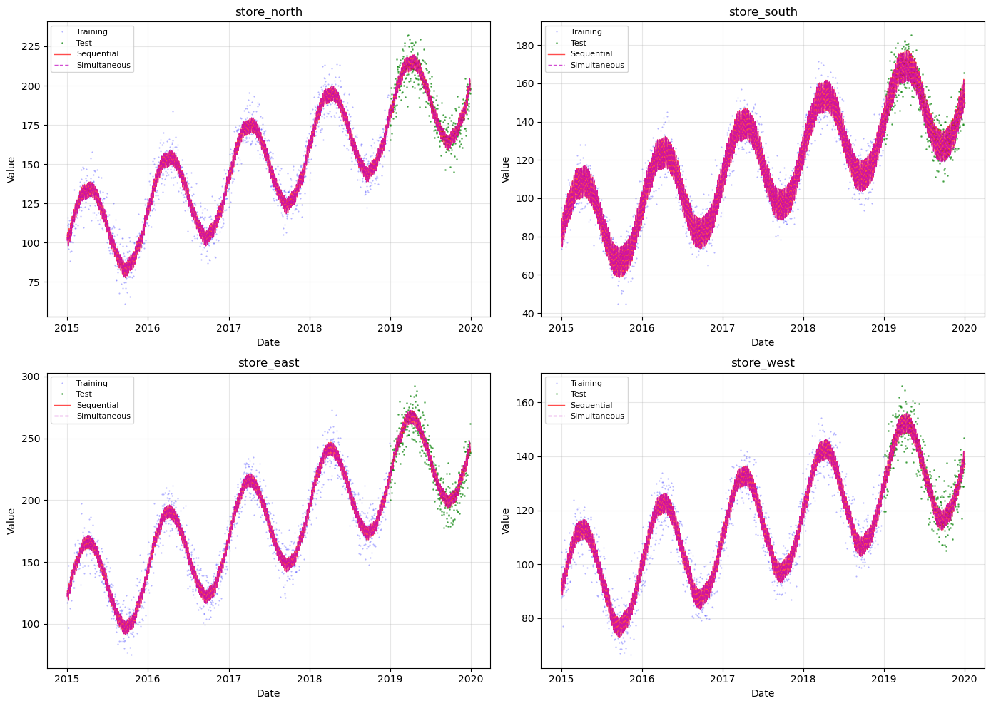
Comparison of Results#
Let’s compare the two approaches side by side.
[14]:
# Timing comparison
timing_comparison = pd.DataFrame(
    {
        "Approach": ["Sequential (Prophet-style)", "Simultaneous (Vangja-style)"],
        "Time (s)": [total_sequential_time, time_combined],
        "Speedup": [1.0, total_sequential_time / time_combined],
    }
)

print("Timing Comparison:")
display(timing_comparison)
Timing Comparison:
| Approach | Time (s) | Speedup | |
|---|---|---|---|
| 0 | Sequential (Prophet-style) | 20.214615 | 1.000000 |
| 1 | Simultaneous (Vangja-style) | 5.787260 | 3.492951 |
[15]:
# Metrics comparison
comparison_rows = []
for params in series_params:
    name = params["name"]
    seq_metrics = sequential_metrics_df.loc[name]
    sim_metrics = simultaneous_metrics_df.loc[name]

    comparison_rows.append(
        {
            "Series": name,
            "Approach": "Sequential",
            "RMSE": seq_metrics["rmse"],
            "MAE": seq_metrics["mae"],
            "MAPE": seq_metrics["mape"],
        }
    )
    comparison_rows.append(
        {
            "Series": name,
            "Approach": "Simultaneous",
            "RMSE": sim_metrics["rmse"],
            "MAE": sim_metrics["mae"],
            "MAPE": sim_metrics["mape"],
        }
    )

metrics_comparison = pd.DataFrame(comparison_rows)
print("Metrics Comparison:")
display(metrics_comparison)
Metrics Comparison:
| Series | Approach | RMSE | MAE | MAPE | |
|---|---|---|---|---|---|
| 0 | store_north | Sequential | 8.098725 | 6.450520 | 0.034214 |
| 1 | store_north | Simultaneous | 8.092538 | 6.444646 | 0.034175 |
| 2 | store_south | Sequential | 6.337769 | 5.071716 | 0.034952 |
| 3 | store_south | Simultaneous | 6.325566 | 5.062452 | 0.034804 |
| 4 | store_east | Sequential | 9.604767 | 7.644443 | 0.033662 |
| 5 | store_east | Simultaneous | 9.619677 | 7.663854 | 0.033768 |
| 6 | store_west | Sequential | 5.363435 | 4.284655 | 0.031891 |
| 7 | store_west | Simultaneous | 5.357389 | 4.277841 | 0.031851 |
| 8 | store_central | Sequential | 11.448755 | 9.184140 | 0.032899 |
| 9 | store_central | Simultaneous | 11.437660 | 9.175294 | 0.032854 |
[16]:
# Visual comparison for a few series
fig, axes = plt.subplots(2, 2, figsize=(14, 10))
axes = axes.flatten()

for i, (ax, params) in enumerate(zip(axes, series_params[:4])):
    name = params["name"]
    train_df = train_series[i]
    test_df = test_series[i]

    # Sequential prediction
    future_seq = sequential_futures[i]

    # Simultaneous prediction
    group_code = [k for k, v in model_combined.groups_.items() if v == name][0]

    ax.plot(
        train_df["ds"], train_df["y"], "b.", markersize=1, alpha=0.3, label="Training"
    )
    ax.plot(test_df["ds"], test_df["y"], "g.", markersize=2, alpha=0.5, label="Test")
    ax.plot(
        future_seq["ds"],
        future_seq["yhat_0"],
        "r-",
        linewidth=1,
        alpha=0.7,
        label="Sequential",
    )
    ax.plot(
        future_combined["ds"],
        future_combined[f"yhat_{group_code}"],
        "m--",
        linewidth=1,
        alpha=0.7,
        label="Simultaneous",
    )

    ax.set_title(name)
    ax.set_xlabel("Date")
    ax.set_ylabel("Value")
    ax.legend(loc="upper left", fontsize=8)
    ax.grid(True, alpha=0.3)

plt.tight_layout()
plt.show()
Summary#
Key Findings#
Equivalent Results: When all series share the same time range, sequential and simultaneous fitting produce nearly identical results. Small differences are due to optimization randomness.
Significant Speedup: Simultaneous fitting is substantially faster due to:
Single model compilation (vs. N separate compilations)
Vectorized JAX computations across all series
The speedup increases with more time series
Scalability: While we demonstrated with 5 series, vangja can handle hundreds of time series simultaneously, making it ideal for:
Retail demand forecasting (many SKUs)
Energy load forecasting (many meters)
Financial time series (many stocks)
When to Use Simultaneous Fitting#
Scenario |
Recommendation |
|---|---|
Many series, same time range |
✅ Use simultaneous fitting |
Few series (<3) |
Either approach works |
Different model per series |
Use sequential fitting |
Series with different date ranges |
See Chapter 04 for caveats |
Important Caveats#
Simultaneous fitting works best when series share the same time range. When fitting series with very different date ranges (e.g., 1949-1960 vs 2007-2016), there are important considerations:
Changepoint placement: The
n_changepointsare distributed across the entire combined time range, so each individual series may get fewer changepoints than expectedTime normalization: Each series occupies only a portion of
t = [0, 1]Prediction filtering: You must filter predictions to each series’ relevant date range
See Chapter 04: Multi-Series Fitting Caveats for detailed examples and solutions.
What’s Next#
Chapter 04 examines what happens when the time series being fitted simultaneously have different date ranges — a common real-world scenario that introduces subtle but important pitfalls.