Chapter 06: Caveats of Hierarchical Modeling#
In the previous chapter we saw how partial pooling allows related series to share seasonal information through a hierarchical structure, producing coherent predictions even in data gaps. In this chapter, we explore two important caveats of hierarchical modeling as implemented in vangja (following the timeseers approach):
Shrinkage strength is a hyperparameter — The
shrinkage_strengthparameter controls how strongly individual series are pulled toward the shared mean. Different values produce different results, and there is no universal default. This parameter must be tuned for each problem.Opposite seasonality and the UniformConstant trick — The timeseers library proposes using
UniformConstant(-1, 1)as a multiplicative factor on seasonality to handle series with opposite seasonal patterns (e.g., summer vs winter products). We investigate whether this is necessary or whether partial pooling on the Fourier coefficients already handles opposite seasonality implicitly.
Setup and Imports#
[1]:
import warnings

warnings.filterwarnings("ignore")
[2]:
import time

import matplotlib.pyplot as plt
import numpy as np
import pandas as pd

from vangja import FourierSeasonality, LinearTrend, UniformConstant
from vangja.datasets import generate_hierarchical_products
from vangja.utils import metrics, remove_random_gaps

print("Imports successful!")
Imports successful!
Data Generation#
We use the same data generation process as in Chapter 05: synthetic products with summer/winter seasonality and random gaps.
[3]:
# Same data generation as Chapter 05
df_full, product_params = generate_hierarchical_products(seed=42, include_all_year=True)

np.random.seed(42)
df_parts = []
for name, params in product_params.items():
    series_data = df_full[df_full["series"] == name].copy()
    if params["group"] != "all_year":
        series_data = remove_random_gaps(series_data, n_gaps=4, gap_fraction=0.2)
    df_parts.append(series_data)

df = pd.concat(df_parts, ignore_index=True)

print(f"Date range: {df['ds'].min().date()} to {df['ds'].max().date()}")
print(f"Products: {list(product_params.keys())}")
for name, params in product_params.items():
    n = len(df[df["series"] == name])
    print(f"  {name} ({params['group']}): {n} points")
Date range: 2018-01-01 to 2019-12-31
Products: ['summer_1', 'summer_2', 'summer_3', 'winter_1', 'winter_2', 'all_year']
  summer_1 (summer): 292 points
  summer_2 (summer): 146 points
  summer_3 (summer): 146 points
  winter_1 (winter): 146 points
  winter_2 (winter): 292 points
  all_year (all_year): 730 points
Caveat 1: Shrinkage Strength#
The shrinkage_strength parameter controls how strongly individual series parameters are pulled toward the shared group mean. In the hierarchical structure:
Higher shrinkage_strength means the prior on \(\beta_{\sigma}\) is tighter around zero, so individual series are pulled more strongly toward \(\beta_{\text{shared}}\).
Low shrinkage (e.g., 1): Each series can deviate freely from the shared mean → closer to individual fitting
High shrinkage (e.g., 1000): Series are forced to be very similar → closer to complete pooling
There is no universal best value — it depends on how similar the series truly are. This is a hyperparameter that must be tuned for each problem, typically via cross-validation or domain knowledge.
Let’s fit partial pooling models with different shrinkage strengths on the yearly seasonality (keeping trend shrinkage fixed at 10) and compare the results.
[4]:
shrinkage_values = [1, 10, 100, 1000, 10000]
shrinkage_models = {}
shrinkage_predictions = {}

for shrinkage in shrinkage_values:
    print(f"\nFitting with shrinkage_strength={shrinkage}...")
    model = (
        LinearTrend(
            n_changepoints=10,
            pool_type="partial",
            delta_pool_type="partial",
            shrinkage_strength=10,  # Fixed trend shrinkage
        )
        + FourierSeasonality(
            period=365.25,
            series_order=5,
            pool_type="partial",
            shrinkage_strength=shrinkage,
        )
        + FourierSeasonality(
            period=7,
            series_order=2,
            pool_type="partial",
            shrinkage_strength=shrinkage,
        )
    )

    start = time.time()
    model.fit(df, method="mapx", scale_mode="individual", sigma_pool_type="individual")
    elapsed = time.time() - start
    future = model.predict(horizon=0, freq="D")

    shrinkage_models[shrinkage] = model
    shrinkage_predictions[shrinkage] = future
    print(f"  Done in {elapsed:.2f}s")
Fitting with shrinkage_strength=1...
WARNING:2026-02-27 00:16:19,660:jax._src.xla_bridge:876: An NVIDIA GPU may be present on this machine, but a CUDA-enabled jaxlib is not installed. Falling back to cpu.
  Done in 16.49s

Fitting with shrinkage_strength=10...
  Done in 26.11s

Fitting with shrinkage_strength=100...
  Done in 10.54s

Fitting with shrinkage_strength=1000...
  Done in 12.40s

Fitting with shrinkage_strength=10000...
Done in 25.07s
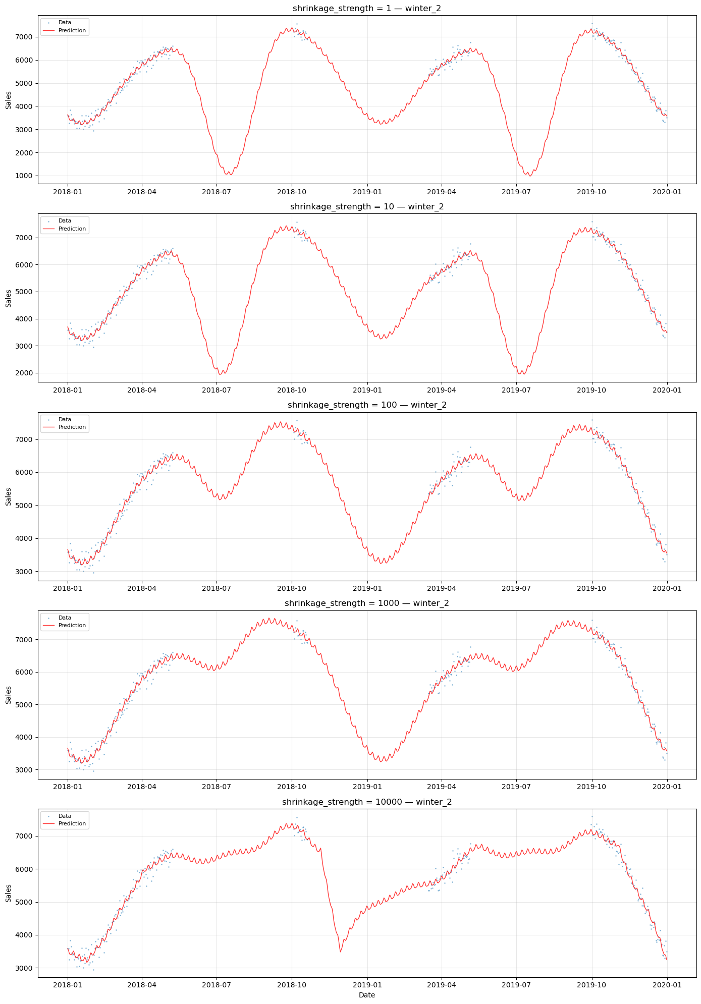
[5]:
# Compare predictions for winter_2 across shrinkage values
# This series has opposite (winter) seasonality and data gaps
series_name = "winter_2"
series_data = df[df["series"] == series_name]

fig, axes = plt.subplots(
    len(shrinkage_values), 1, figsize=(14, 4 * len(shrinkage_values))
)

for ax, shrinkage in zip(axes, shrinkage_values):
    model = shrinkage_models[shrinkage]
    future = shrinkage_predictions[shrinkage]
    group_code = [k for k, v in model.groups_.items() if v == series_name][0]

    ax.scatter(
        series_data["ds"], series_data["y"], s=1, alpha=0.4, color="C0", label="Data"
    )
    ax.plot(
        future["ds"],
        future[f"yhat_{group_code}"],
        "r-",
        linewidth=1,
        alpha=0.8,
        label="Prediction",
    )
    ax.set_title(f"shrinkage_strength = {shrinkage} — {series_name}")
    ax.set_ylabel("Sales")
    ax.legend(loc="upper left", fontsize=8)
    ax.grid(True, alpha=0.3)

axes[-1].set_xlabel("Date")
plt.tight_layout()
plt.show()
[6]:
# Compare predictions for all_year across shrinkage values
# This series has complete data and minimal seasonality
series_name = "all_year"
series_data = df[df["series"] == series_name]

fig, axes = plt.subplots(
    len(shrinkage_values), 1, figsize=(14, 4 * len(shrinkage_values))
)

for ax, shrinkage in zip(axes, shrinkage_values):
    model = shrinkage_models[shrinkage]
    future = shrinkage_predictions[shrinkage]
    group_code = [k for k, v in model.groups_.items() if v == series_name][0]

    ax.scatter(
        series_data["ds"], series_data["y"], s=1, alpha=0.4, color="C0", label="Data"
    )
    ax.plot(
        future["ds"],
        future[f"yhat_{group_code}"],
        "r-",
        linewidth=1,
        alpha=0.8,
        label="Prediction",
    )
    ax.set_title(f"shrinkage_strength = {shrinkage} — {series_name}")
    ax.set_ylabel("Sales")
    ax.legend(loc="upper left", fontsize=8)
    ax.grid(True, alpha=0.3)

axes[-1].set_xlabel("Date")
plt.tight_layout()
plt.show()
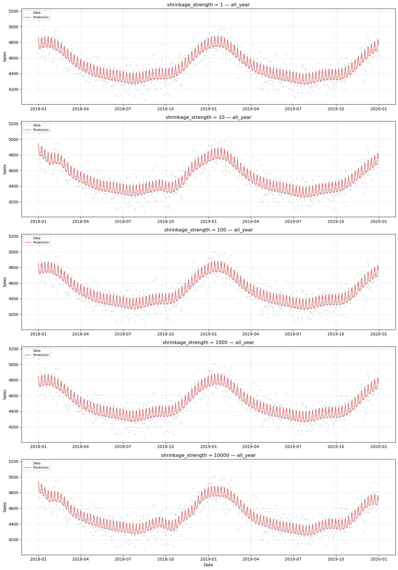
Observations#
Low shrinkage (1): Each series has near-complete freedom to learn its own seasonal pattern. This is close to individual fitting — the model may produce erratic predictions in data gaps because there is minimal information sharing.
Moderate shrinkage (10–100): A balance between sharing and individuality. The shared seasonal pattern provides a reasonable baseline, while individual deviations capture series-specific differences.
High shrinkage (1000): Series are forced to have very similar seasonal patterns.
The optimal shrinkage depends on:
How similar the seasonal patterns truly are across series
How much data each series has (less data → more benefit from sharing)
Whether the series have opposite seasonality (which complicates the shared mean)
Bottom line: shrinkage_strength is a hyperparameter that must be tuned. Cross-validation or Bayesian model comparison (e.g., LOO-CV, WAIC) can help select an appropriate value.
Caveat 2: Opposite Seasonality and the UniformConstant#
The timeseers library proposes a clever pattern for handling series with opposite seasonal patterns under partial pooling: multiply the seasonality by a UniformConstant(-1, 1):
model = (
    LinearTrend()
    + UniformConstant(-1, 1) * FourierSeasonality(365.25, 5)
    + FourierSeasonality(7, 2)
)
The idea is that the constant learns:
\(c \approx +1\) for summer products (keep the seasonal pattern as-is)
\(c \approx -1\) for winter products (flip the seasonal pattern)
\(c \approx 0\) for all-year products (suppress seasonality)
Why might this be necessary?#
Consider what happens with partial pooling on Fourier coefficients when series have opposite seasonality.
Without UniformConstant:
Summer products want positive \(\beta\), winter products want negative \(\beta\). The shared mean \(\beta_{\text{shared}}\) is pulled in both directions and compromises near zero. With high shrinkage (small \(\beta_{\sigma}\)), individual deviations are forced to be small, so all series end up with weak seasonality.
With UniformConstant:
Now \(\beta_{\text{shared}}\) can represent the magnitude of the seasonal pattern (consistently positive), while \(c_i\) handles the direction (sign). High shrinkage on \(\beta\) works well because all series genuinely share the same seasonal shape — only the direction differs.
Or is the model already handling this implicitly?#
With low to moderate shrinkage on Fourier coefficients, each series’ \(\beta_i\) can deviate enough from \(\beta_{\text{shared}}\) to have opposite signs. The model effectively learns positive coefficients for summer and negative for winter. The sharing benefit is reduced (because \(\beta_{\text{shared}} \approx 0\)), but it still works.
Let’s test both approaches and compare.
Model without UniformConstant (same as Chapter 05)#
This is the same partial pooling model from Chapter 05 with high shrinkage on seasonality.
[7]:
# Partial pooling without UniformConstant (from Chapter 05)
model_no_uc = (
    LinearTrend(
        n_changepoints=10,
        pool_type="partial",
        delta_pool_type="partial",
        shrinkage_strength=10,
    )
    + FourierSeasonality(
        period=365.25, series_order=5, pool_type="partial", shrinkage_strength=1000
    )
    + FourierSeasonality(
        period=7, series_order=2, pool_type="partial", shrinkage_strength=1000
    )
)

start = time.time()
model_no_uc.fit(
    df, method="mapx", scale_mode="individual", sigma_pool_type="individual"
)
time_no_uc = time.time() - start

future_no_uc = model_no_uc.predict(horizon=0, freq="D")
print(f"Without UniformConstant: {time_no_uc:.2f}s")
Without UniformConstant: 11.63s
Model with UniformConstant (timeseers pattern)#
Now we add UniformConstant(-1, 1) as a multiplicative factor on the yearly seasonality. The constant is partially pooled so each series can learn its own direction. All other parameters remain the same.
[8]:
# Partial pooling with UniformConstant (timeseers pattern)
model_uc = (
    LinearTrend(
        n_changepoints=10,
        pool_type="partial",
        delta_pool_type="partial",
        shrinkage_strength=10,
    )
    + UniformConstant(-1, 1, pool_type="individual")
    ** FourierSeasonality(
        period=365.25, series_order=5, pool_type="partial", shrinkage_strength=1000
    )
    + FourierSeasonality(
        period=7, series_order=2, pool_type="partial", shrinkage_strength=1000
    )
)

start = time.time()
model_uc.fit(df, method="mapx", scale_mode="individual", sigma_pool_type="individual")
time_uc = time.time() - start

future_uc = model_uc.predict(horizon=0, freq="D")
print(f"With UniformConstant: {time_uc:.2f}s")
With UniformConstant: 19.89s
Comparing the two approaches#
Let’s use the built-in plot() method to see the component decomposition for a winter product. This shows how each model handles the opposite seasonality.
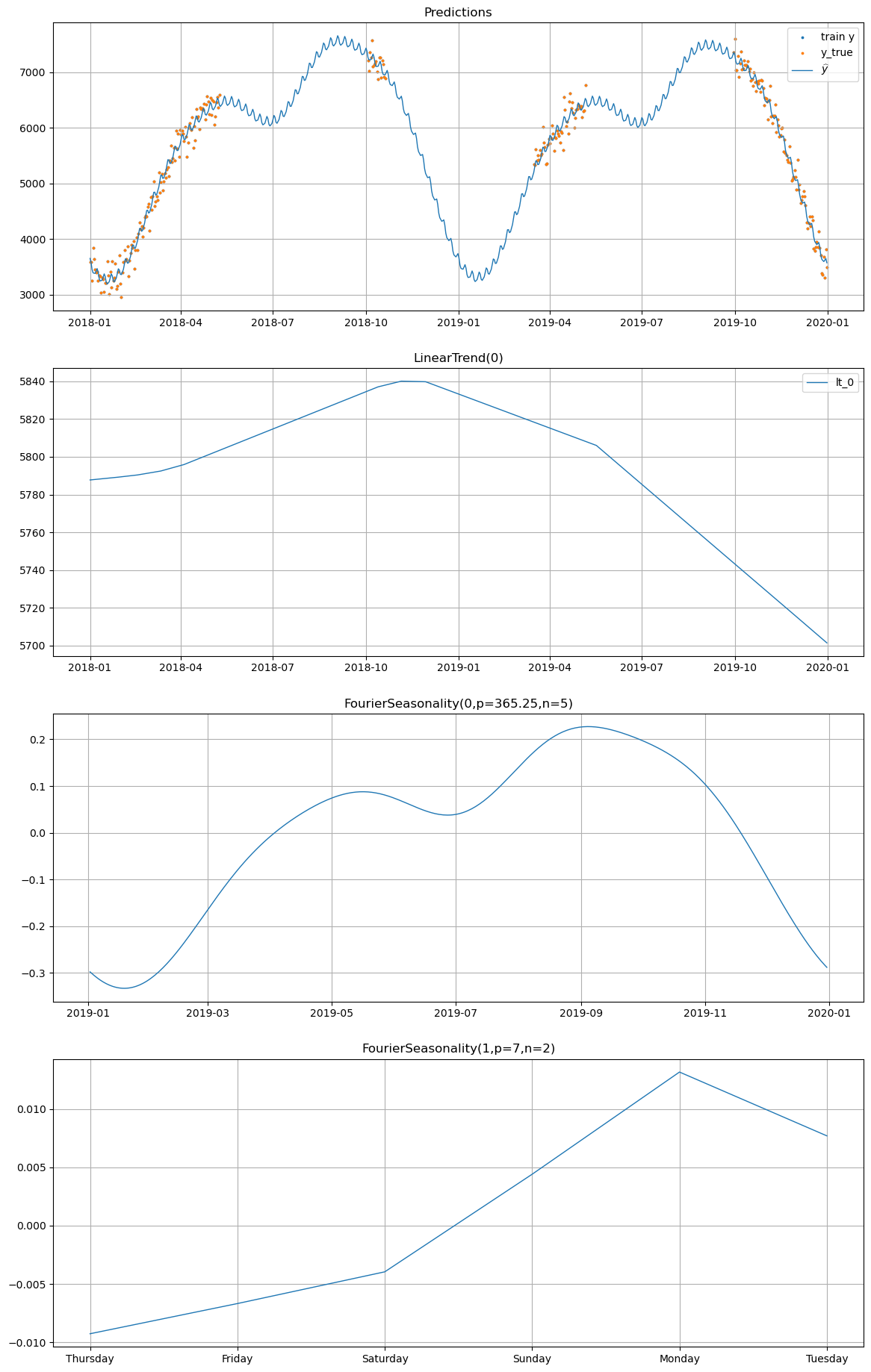
[9]:
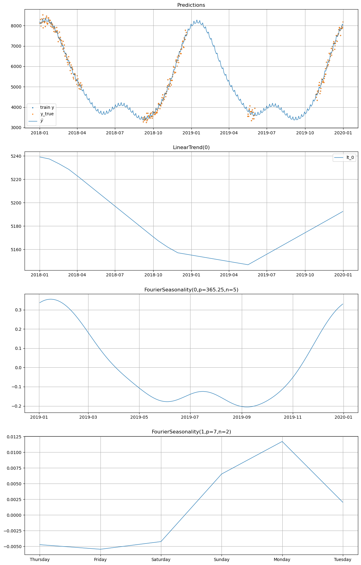
# Plot decomposition for winter_2 WITHOUT UniformConstant
print("=== Without UniformConstant ===")
model_no_uc.plot(future_no_uc, series="winter_2", y_true=df[df["series"] == "winter_2"])
=== Without UniformConstant ===
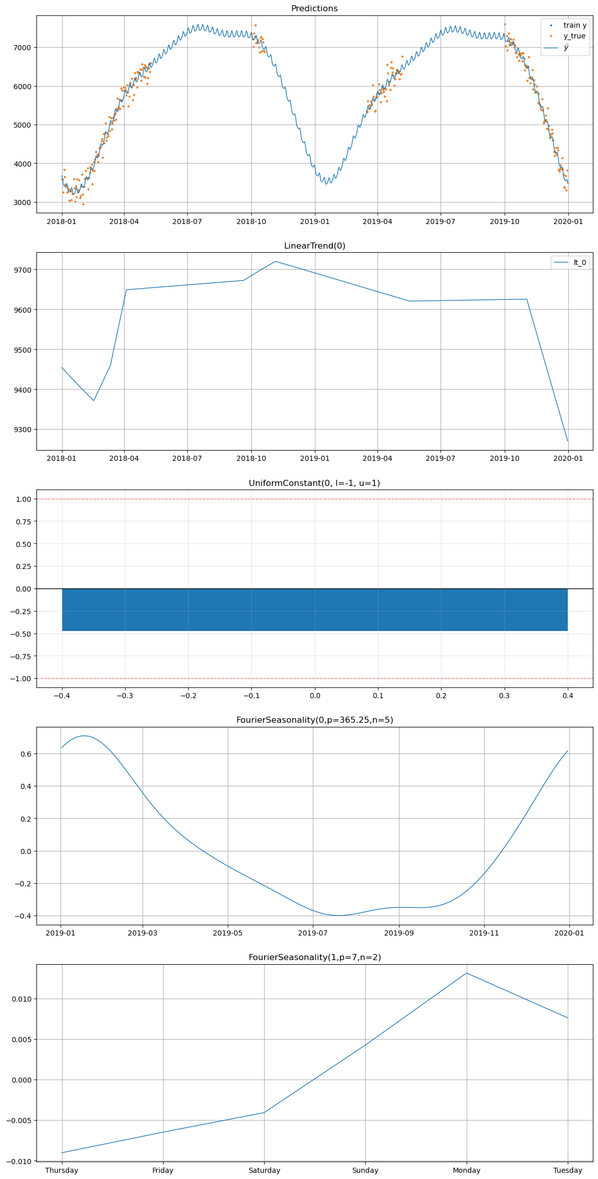
[10]:
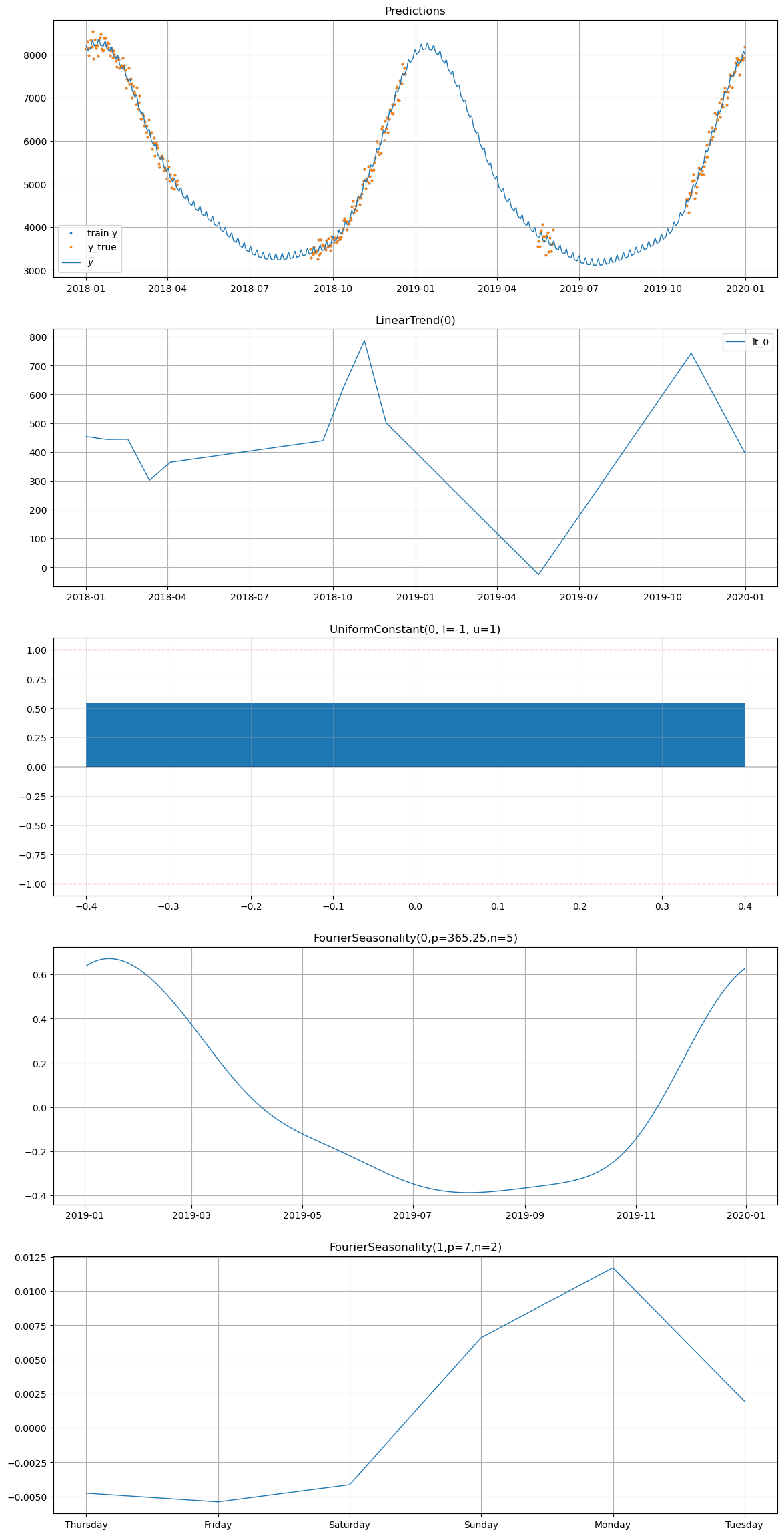
# Plot decomposition for winter_2 WITH UniformConstant
print("=== With UniformConstant ===")
model_uc.plot(future_uc, series="winter_2", y_true=df[df["series"] == "winter_2"])
=== With UniformConstant ===
[11]:
# Plot decomposition for summer_1 WITHOUT UniformConstant
print("=== Without UniformConstant ===")
model_no_uc.plot(future_no_uc, series="summer_1", y_true=df[df["series"] == "summer_1"])
=== Without UniformConstant ===
[12]:
# Plot decomposition for summer_1 WITH UniformConstant
print("=== With UniformConstant ===")
model_uc.plot(future_uc, series="summer_1", y_true=df[df["series"] == "summer_1"])
=== With UniformConstant ===
[13]:
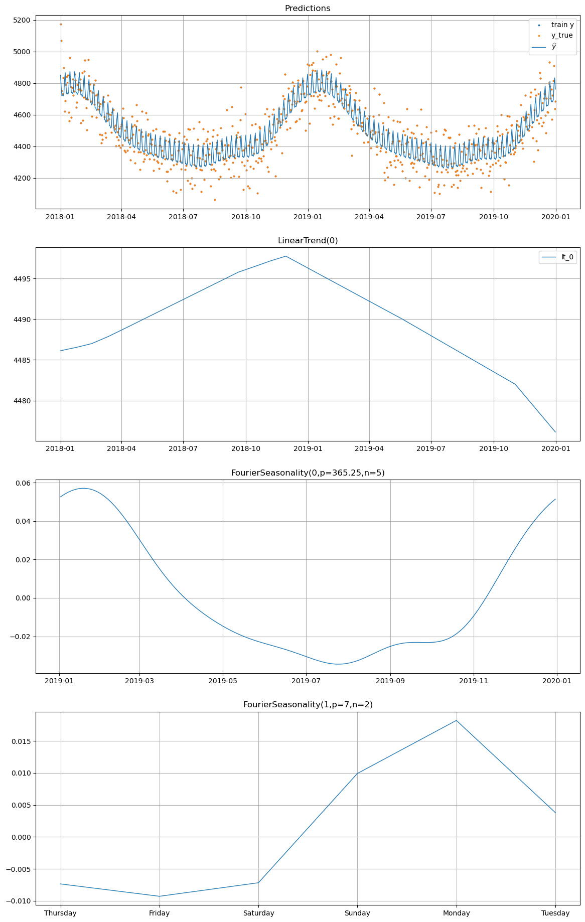
# Plot decomposition for all_year WITHOUT UniformConstant
print("=== Without UniformConstant ===")
model_no_uc.plot(future_no_uc, series="all_year", y_true=df[df["series"] == "all_year"])
=== Without UniformConstant ===
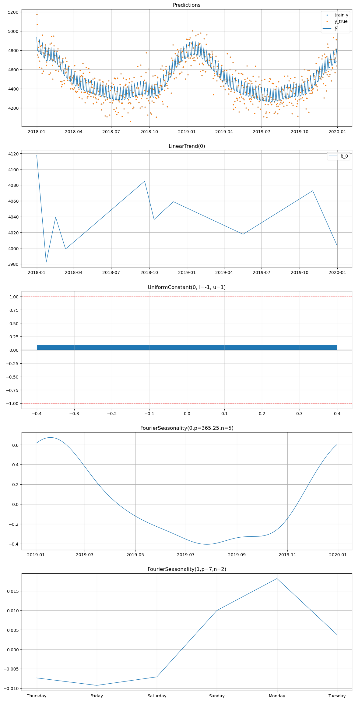
[14]:
# Plot decomposition for all_year WITH UniformConstant
print("=== With UniformConstant ===")
model_uc.plot(future_uc, series="all_year", y_true=df[df["series"] == "all_year"])
=== With UniformConstant ===
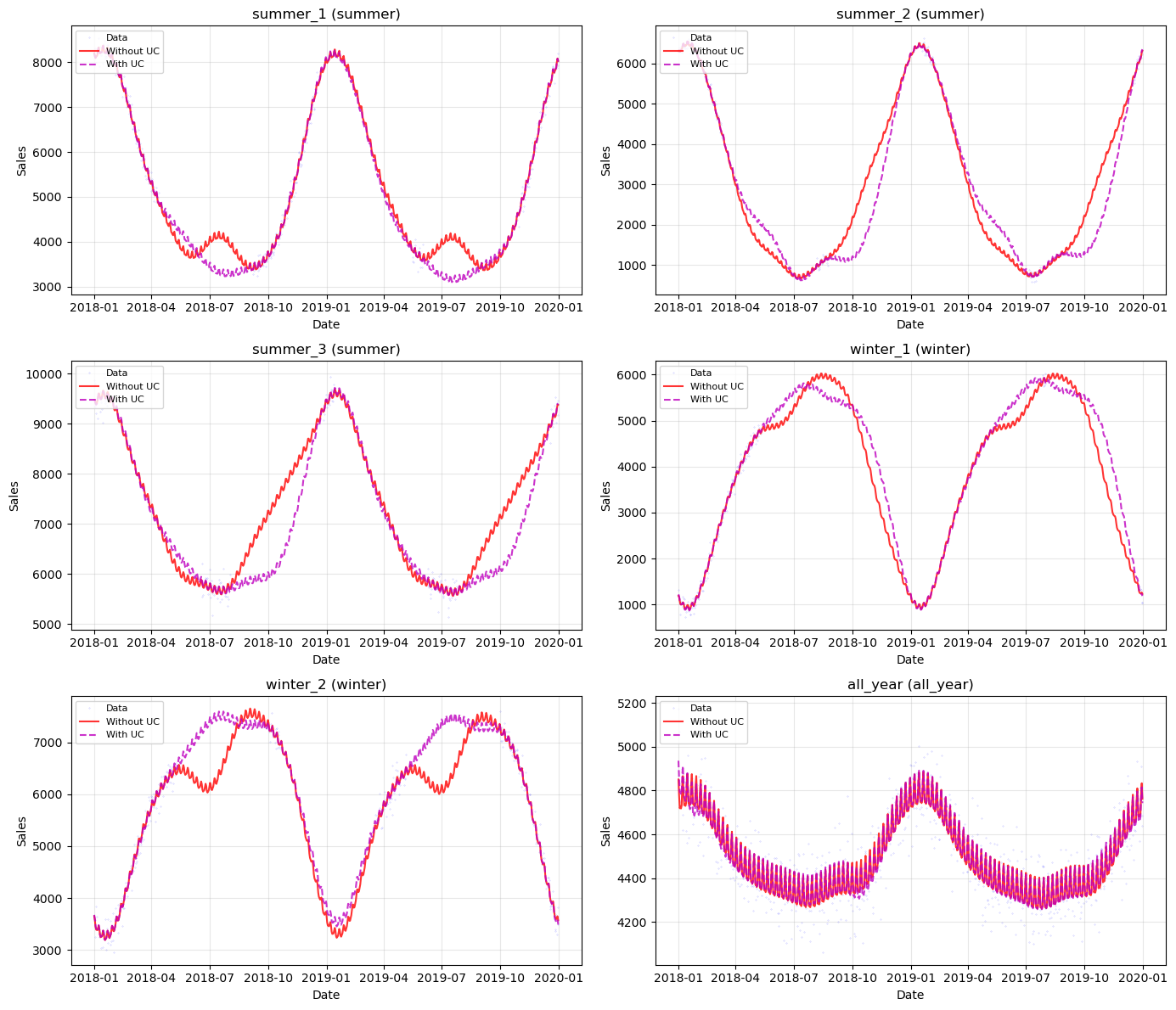
Side-by-side comparison for all series#
[15]:
# Overlay predictions from both models for all series
fig, axes = plt.subplots(3, 2, figsize=(14, 12))
axes = axes.flatten()

for i, (name, params) in enumerate(product_params.items()):
    ax = axes[i]
    series_data = df[df["series"] == name]

    no_uc_group = [k for k, v in model_no_uc.groups_.items() if v == name][0]
    uc_group = [k for k, v in model_uc.groups_.items() if v == name][0]

    ax.plot(
        series_data["ds"],
        series_data["y"],
        "b.",
        markersize=0.5,
        alpha=0.3,
        label="Data",
    )
    ax.plot(
        future_no_uc["ds"],
        future_no_uc[f"yhat_{no_uc_group}"],
        "r-",
        linewidth=1.5,
        alpha=0.8,
        label="Without UC",
    )
    ax.plot(
        future_uc["ds"],
        future_uc[f"yhat_{uc_group}"],
        "m--",
        linewidth=1.5,
        alpha=0.8,
        label="With UC",
    )

    ax.set_title(f"{name} ({params['group']})")
    ax.set_xlabel("Date")
    ax.set_ylabel("Sales")
    ax.legend(loc="upper left", fontsize=8)
    ax.grid(True, alpha=0.3)

plt.tight_layout()
plt.show()
[16]:
# In-sample metrics comparison
comparison_rows = []

for approach_name, model, future in [
    ("Without UC", model_no_uc, future_no_uc),
    ("With UC", model_uc, future_uc),
]:
    for name in product_params.keys():
        group_code = [k for k, v in model.groups_.items() if v == name][0]
        series_data = df[df["series"] == name]
        future_for_metrics = future[["ds", f"yhat_{group_code}"]].copy()
        future_for_metrics.columns = ["ds", "yhat_0"]
        m = metrics(series_data, future_for_metrics, "complete")
        comparison_rows.append(
            {
                "Series": name,
                "Group": product_params[name]["group"],
                "Approach": approach_name,
                "RMSE": m["rmse"].values[0],
                "MAE": m["mae"].values[0],
                "MAPE": m["mape"].values[0],
            }
        )

comparison_df = pd.DataFrame(comparison_rows)
print("Metrics Comparison:")
display(comparison_df)

print("\nSummary by Approach:")
display(
    comparison_df.groupby("Approach")
    .agg({"RMSE": ["mean", "std"], "MAE": ["mean", "std"]})
    .round(2)
)
Metrics Comparison:
| Series | Group | Approach | RMSE | MAE | MAPE | |
|---|---|---|---|---|---|---|
| 0 | summer_1 | summer | Without UC | 142.152841 | 114.761139 | 0.020943 |
| 1 | summer_2 | summer | Without UC | 91.518750 | 74.878657 | 0.032018 |
| 2 | summer_3 | summer | Without UC | 186.977001 | 146.326295 | 0.021774 |
| 3 | winter_1 | winter | Without UC | 112.821920 | 93.404084 | 0.049773 |
| 4 | winter_2 | winter | Without UC | 166.712894 | 131.774282 | 0.026323 |
| 5 | all_year | all_year | Without UC | 100.746479 | 79.753239 | 0.017812 |
| 6 | summer_1 | summer | With UC | 140.464419 | 113.067301 | 0.020632 |
| 7 | summer_2 | summer | With UC | 89.862287 | 73.439107 | 0.031606 |
| 8 | summer_3 | summer | With UC | 186.548404 | 145.914661 | 0.021720 |
| 9 | winter_1 | winter | With UC | 110.110254 | 90.501832 | 0.048353 |
| 10 | winter_2 | winter | With UC | 164.963507 | 129.342518 | 0.025819 |
| 11 | all_year | all_year | With UC | 99.800278 | 79.535853 | 0.017768 |
Summary by Approach:
| RMSE | MAE | |||
|---|---|---|---|---|
| mean | std | mean | std | |
| Approach | ||||
| With UC | 131.96 | 38.54 | 105.30 | 28.93 |
| Without UC | 133.49 | 38.21 | 106.82 | 28.91 |
Analysis#
Without UniformConstant: The partial pooling model with high shrinkage on the Fourier coefficients (\(\text{shrinkage\_strength} = 1000\)) forces the shared seasonal mean \(\beta_{\text{shared}}\) close to zero, because summer and winter products pull in opposite directions. The individual deviations \(\beta_{\sigma}\) must compensate, but their prior is very tight. As a result, the model may produce weaker seasonal patterns, or the optimizer may find a solution where the seasonal signal is partly absorbed into the trend or noise.
With UniformConstant: The constant \(c_i\) absorbs the sign difference between groups. Summer products learn \(c \approx +1\), winter products learn \(c \approx -1\), and the all-year product learns \(c \approx 0\). This means \(\beta_{\text{shared}}\) can represent the actual seasonal shape (magnitude and phase), and high shrinkage genuinely forces series to share the same seasonal shape — the intended behavior.
Conclusion#
The results reveal important insights about how partial pooling handles opposite seasonality. The UniformConstant trick is not strictly necessary — partial pooling can handle opposite seasonality by allowing individual deviations to have opposite signs. However, it becomes increasingly valuable as shrinkage strength increases:
Shrinkage |
Without UC |
With UC |
|---|---|---|
Low (1-10) |
Works fine — individual betas can freely deviate |
Adds complexity with little benefit |
Moderate (10-100) |
May weaken some seasonal patterns |
Better separation of shape vs direction |
High (100-1000) |
Shared mean ≈ 0, weak seasonality |
Shared shape is meaningful, direction via constant |
The UniformConstant approach is most useful when:
You have series with genuinely opposite seasonality (not just different amplitudes)
You want strong shrinkage to share seasonal shape across series
The seasonal shape is similar across groups but the direction differs
If your series have simply different (not opposite) seasonal patterns, the UniformConstant adds unnecessary complexity and you are better off with lower shrinkage on the Fourier coefficients directly.
Summary#
Hierarchical modeling with partial pooling is a powerful technique, but it comes with important caveats:
Shrinkage strength is a hyperparameter. There is no universal default. Too little shrinkage gives up the sharing benefit; too much forces series to be more similar than they truly are. Tune it via cross-validation or domain knowledge.
Opposite seasonality requires care. When series have opposite seasonal patterns, the shared Fourier coefficients are pulled toward zero under high shrinkage. The
UniformConstant(-1, 1)trick from timeseers elegantly separates seasonal shape from seasonal direction, enabling strong shrinkage on the shape while allowing the direction to vary per series. Without it, the model can still work with lower shrinkage, but the sharing benefit is reduced.
These caveats are not weaknesses — they are inherent to any hierarchical model. Understanding them helps practitioners make informed modeling choices rather than blindly applying defaults.
What’s Next#
In Chapter 07, we move from sharing information across series to sharing information across time — introducing transfer learning from a long time series to a short one. This is vangja’s most distinctive feature.