Chapter 10: Bayesian Workflow — Diagnostics and Best Practices#
This chapter brings together the transfer learning scenario from Chapters 07–08 and augments it with the diagnostic steps recommended by the WAMBS (When to Worry and how to Avoid the Misuse of Bayesian Statistics) checklist.
In This Notebook#
Prior predictive checks — Do the priors produce plausible data before fitting?
Convergence diagnostics — R-hat, ESS, trace plots, energy plots
Posterior predictive checks — Does the fitted model generate data that looks like the observations?
Model comparison — WAIC / LOO-CV between baseline and transfer models
Prior sensitivity analysis — How sensitive are forecasts to prior choices?
Full posterior summaries — HDI, credible intervals, not just point estimates
Prior-to-posterior visualisation — Showing how the data updates our beliefs
These are not optional extras — they are the core of responsible Bayesian analysis.
Setup and Imports#
[1]:
import warnings

warnings.filterwarnings("ignore")
[2]:
import arviz as az
import matplotlib.pyplot as plt
import numpy as np
import pandas as pd

from vangja import FlatTrend, FourierSeasonality, LinearTrend
from vangja.datasets import load_citi_bike_sales, load_nyc_temperature
from vangja.utils import (
    metrics,
    plot_posterior_predictive,
    plot_prior_posterior,
    plot_prior_predictive,
    prior_sensitivity_analysis,
)

az.style.use("arviz-darkgrid")

np.random.seed(42)

print("Imports successful!")
Imports successful!
1. Data Loading#
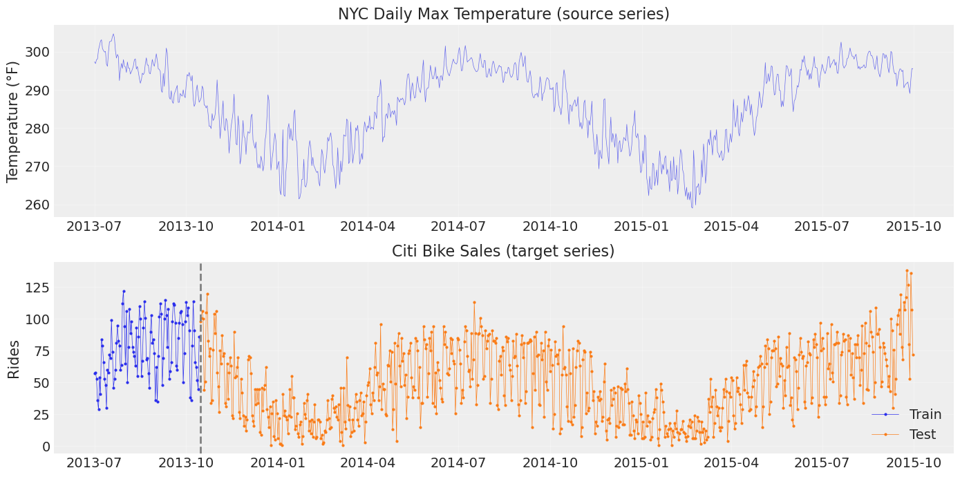
We reproduce the setup from Chapter 07: a long NYC temperature series (source) and a short Citi Bike sales series (target with ~3 months training data).
[3]:
# Load datasets
temp_df = load_nyc_temperature()
sales_df = load_citi_bike_sales()

# Match date ranges as in the original blog post
temp_df = temp_df[
    (temp_df["ds"] >= sales_df["ds"].min()) & (temp_df["ds"] <= sales_df["ds"].max())
]

# Train/test split for sales
train_test_date = pd.to_datetime("2013-10-15")
sales_train = sales_df[sales_df["ds"] < train_test_date].copy()
sales_test = sales_df[sales_df["ds"] >= train_test_date].copy()

print(
    f"Temperature: {temp_df.shape[0]} days  ({temp_df['ds'].min().date()} – {temp_df['ds'].max().date()})"
)
print(
    f"Sales train: {sales_train.shape[0]} days ({sales_train['ds'].min().date()} – {sales_train['ds'].max().date()})"
)
print(
    f"Sales test:  {sales_test.shape[0]} days ({sales_test['ds'].min().date()} – {sales_test['ds'].max().date()})"
)
Temperature: 822 days  (2013-07-01 – 2015-09-30)
Sales train: 106 days (2013-07-01 – 2013-10-14)
Sales test:  716 days (2013-10-15 – 2015-09-30)
[4]:
fig, axes = plt.subplots(2, 1, figsize=(14, 7))

axes[0].plot(temp_df["ds"], temp_df["y"], "C0-", lw=0.5, alpha=0.7)
axes[0].set_title("NYC Daily Max Temperature (source series)")
axes[0].set_ylabel("Temperature (°F)")

axes[1].plot(sales_train["ds"], sales_train["y"], "C0o-", ms=2, lw=0.5, label="Train")
axes[1].plot(sales_test["ds"], sales_test["y"], "C1o-", ms=2, lw=0.5, label="Test")
axes[1].axvline(train_test_date, color="gray", ls="--", lw=2)
axes[1].set_title("Citi Bike Sales (target series)")
axes[1].set_ylabel("Rides")
axes[1].legend()

for ax in axes:
    ax.grid(True, alpha=0.3)
plt.tight_layout()
plt.show()
2. Prior Predictive Checks#
Why? Before fitting, we should verify that our priors produce data in a plausible range. If the prior predictive distribution generates wildly unreasonable values, our priors need adjustment. This is the first step in the WAMBS checklist.
We compare prior predictives from:
A baseline model (default uninformed priors)
The temperature model (simple priors, long data)
2.1 Temperature Model — Prior Predictive#
[5]:
# Define the temperature model
temp_model = FlatTrend() + FourierSeasonality(period=365.25, series_order=6)

# We need to fit first to build the PyMC model graph, then sample from the prior
# Fit with NUTS for full posterior (needed for diagnostics later)
print("Fitting temperature model with NUTS...")
temp_model.fit(temp_df, method="nuts", scaler="minmax")
print("Done!")
Fitting temperature model with NUTS...
Multiprocess sampling (4 chains in 4 jobs)
NUTS: [ft_0 - intercept, fs_0 - beta(p=365.25,n=6), sigma]
Sampling 4 chains for 1_000 tune and 1_000 draw iterations (4_000 + 4_000 draws total) took 5 seconds.
Done!
[6]:
# Sample from the prior predictive
temp_prior_pred = temp_model.sample_prior_predictive(samples=500)

fig, ax = plt.subplots(figsize=(14, 5))
plot_prior_predictive(
    temp_prior_pred,
    data=temp_model.data,
    n_samples=100,
    ax=ax,
    title="Temperature Model — Prior Predictive Check",
)
plt.tight_layout()
plt.show()

print("Each thin blue line is one draw from the prior.")
print("The orange line is the observed temperature data.")
print("Prior predictive should at least *contain* the observed data range.")
Sampling: [fs_0 - beta(p=365.25,n=6), ft_0 - intercept, obs, sigma]
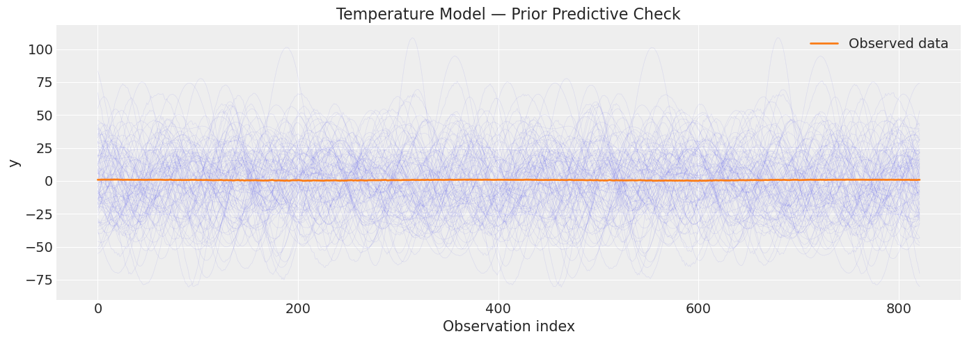
Each thin blue line is one draw from the prior.
The orange line is the observed temperature data.
Prior predictive should at least *contain* the observed data range.
2.2 Baseline Sales Model — Prior Predictive#
The baseline model uses default uninformative priors for yearly seasonality. With only ~3 months of data, the prior predictive may be very wide.
[7]:
# Baseline model (same as Ch07 but fit with NUTS for diagnostics)
baseline_model = (
    LinearTrend(n_changepoints=5)
    + FourierSeasonality(period=365.25, series_order=6)
    + FourierSeasonality(period=91.31, series_order=4)
    + FourierSeasonality(period=30.44, series_order=3)
    + FourierSeasonality(period=7, series_order=2)
)

print("Fitting baseline sales model with NUTS...")
baseline_model.fit(sales_train, method="nuts", scaler="minmax")
print("Done!")
Fitting baseline sales model with NUTS...
Multiprocess sampling (4 chains in 4 jobs)
NUTS: [lt_0 - slope, lt_0 - intercept, lt_0 - delta, fs_0 - beta(p=365.25,n=6), fs_1 - beta(p=91.31,n=4), fs_2 - beta(p=30.44,n=3), fs_3 - beta(p=7,n=2), sigma]
Sampling 4 chains for 1_000 tune and 1_000 draw iterations (4_000 + 4_000 draws total) took 465 seconds.
Chain 0 reached the maximum tree depth. Increase `max_treedepth`, increase `target_accept` or reparameterize.
Chain 1 reached the maximum tree depth. Increase `max_treedepth`, increase `target_accept` or reparameterize.
Chain 2 reached the maximum tree depth. Increase `max_treedepth`, increase `target_accept` or reparameterize.
Chain 3 reached the maximum tree depth. Increase `max_treedepth`, increase `target_accept` or reparameterize.
The rhat statistic is larger than 1.01 for some parameters. This indicates problems during sampling. See https://arxiv.org/abs/1903.08008 for details
The effective sample size per chain is smaller than 100 for some parameters.  A higher number is needed for reliable rhat and ess computation. See https://arxiv.org/abs/1903.08008 for details
Done!
[8]:
baseline_prior_pred = baseline_model.sample_prior_predictive(samples=500)

fig, ax = plt.subplots(figsize=(14, 5))
plot_prior_predictive(
    baseline_prior_pred,
    data=baseline_model.data,
    n_samples=100,
    ax=ax,
    title="Baseline Sales Model — Prior Predictive Check",
)
plt.tight_layout()
plt.show()

print("With default priors, the prior predictive is very diffuse.")
print("This is expected for weakly informative priors.")
Sampling: [fs_0 - beta(p=365.25,n=6), fs_1 - beta(p=91.31,n=4), fs_2 - beta(p=30.44,n=3), fs_3 - beta(p=7,n=2), lt_0 - delta, lt_0 - intercept, lt_0 - slope, obs, sigma]
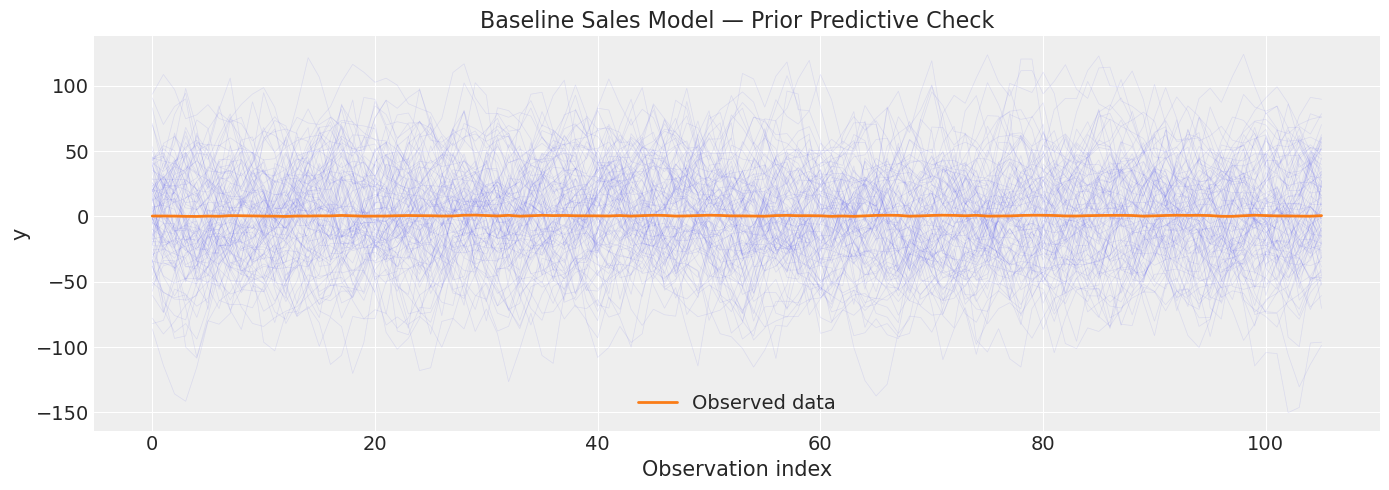
With default priors, the prior predictive is very diffuse.
This is expected for weakly informative priors.
3. Convergence Diagnostics#
After fitting with MCMC, we must verify that the sampler has converged. Key checks:
Diagnostic |
Threshold |
Meaning |
|---|---|---|
R-hat |
< 1.01 |
Chains have mixed well |
ESS bulk |
> 400 |
Enough effective samples for the bulk of the posterior |
ESS tail |
> 400 |
Enough effective samples for the tails |
BFMI |
> 0.3 |
No energy transition problems (NUTS) |
Divergences |
0 |
No pathological geometry |
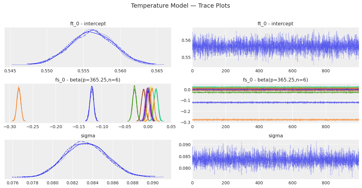
3.1 Temperature Model Convergence#
[9]:
# Convergence summary for the temperature model
temp_summary = temp_model.convergence_summary()
display(temp_summary)

# Check thresholds
rhat_ok = (temp_summary["r_hat"] < 1.01).all()
ess_ok = (temp_summary["ess_bulk"] > 400).all() and (
    temp_summary["ess_tail"] > 400
).all()
print(f"\nR-hat < 1.01 for all parameters: {rhat_ok}")
print(f"ESS > 400 for all parameters:     {ess_ok}")
| mean | sd | hdi_3% | hdi_97% | mcse_mean | mcse_sd | ess_bulk | ess_tail | r_hat | |
|---|---|---|---|---|---|---|---|---|---|
| ft_0 - intercept | 0.556 | 0.003 | 0.550 | 0.562 | 0.0 | 0.0 | 7621.0 | 3391.0 | 1.0 |
| fs_0 - beta(p=365.25,n=6)[0] | -0.122 | 0.004 | -0.130 | -0.114 | 0.0 | 0.0 | 6253.0 | 3072.0 | 1.0 |
| fs_0 - beta(p=365.25,n=6)[1] | -0.280 | 0.004 | -0.287 | -0.272 | 0.0 | 0.0 | 7197.0 | 3238.0 | 1.0 |
| fs_0 - beta(p=365.25,n=6)[2] | -0.029 | 0.004 | -0.037 | -0.021 | 0.0 | 0.0 | 6424.0 | 2636.0 | 1.0 |
| fs_0 - beta(p=365.25,n=6)[3] | -0.001 | 0.004 | -0.009 | 0.007 | 0.0 | 0.0 | 6505.0 | 2794.0 | 1.0 |
| fs_0 - beta(p=365.25,n=6)[4] | -0.010 | 0.004 | -0.017 | -0.001 | 0.0 | 0.0 | 7037.0 | 2915.0 | 1.0 |
| fs_0 - beta(p=365.25,n=6)[5] | 0.018 | 0.004 | 0.010 | 0.026 | 0.0 | 0.0 | 6776.0 | 2997.0 | 1.0 |
| fs_0 - beta(p=365.25,n=6)[6] | 0.004 | 0.004 | -0.003 | 0.012 | 0.0 | 0.0 | 6483.0 | 3069.0 | 1.0 |
| fs_0 - beta(p=365.25,n=6)[7] | 0.018 | 0.004 | 0.010 | 0.026 | 0.0 | 0.0 | 8034.0 | 3409.0 | 1.0 |
| fs_0 - beta(p=365.25,n=6)[8] | -0.002 | 0.004 | -0.009 | 0.006 | 0.0 | 0.0 | 7801.0 | 3041.0 | 1.0 |
| fs_0 - beta(p=365.25,n=6)[9] | 0.002 | 0.004 | -0.006 | 0.010 | 0.0 | 0.0 | 7650.0 | 3330.0 | 1.0 |
| fs_0 - beta(p=365.25,n=6)[10] | 0.000 | 0.004 | -0.008 | 0.008 | 0.0 | 0.0 | 7291.0 | 2852.0 | 1.0 |
| fs_0 - beta(p=365.25,n=6)[11] | 0.009 | 0.004 | 0.001 | 0.016 | 0.0 | 0.0 | 7034.0 | 3003.0 | 1.0 |
| sigma | 0.083 | 0.002 | 0.080 | 0.087 | 0.0 | 0.0 | 6227.0 | 2791.0 | 1.0 |
R-hat < 1.01 for all parameters: True
ESS > 400 for all parameters:     True
[10]:
# Trace plots — visual inspection of mixing
temp_model.plot_trace()
plt.suptitle("Temperature Model — Trace Plots", y=1.02, fontsize=14)
plt.tight_layout()
plt.show()
[11]:
# Energy plot (BFMI diagnostic for NUTS)
temp_model.plot_energy()
plt.suptitle("Temperature Model — Energy Diagnostic", y=1.02)
plt.tight_layout()
plt.show()

print("The marginal energy and energy transition distributions should overlap well.")
print("Large discrepancy indicates the sampler struggles to explore the posterior.")
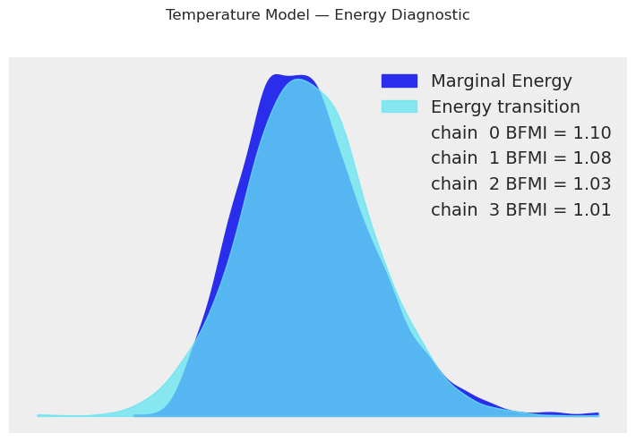
The marginal energy and energy transition distributions should overlap well.
Large discrepancy indicates the sampler struggles to explore the posterior.
3.2 Baseline Sales Model Convergence#
[12]:
baseline_summary = baseline_model.convergence_summary()
display(baseline_summary)

rhat_ok = (baseline_summary["r_hat"] < 1.01).all()
ess_ok = (baseline_summary["ess_bulk"] > 400).all() and (
    baseline_summary["ess_tail"] > 400
).all()
print(f"\nR-hat < 1.01 for all parameters: {rhat_ok}")
print(f"ESS > 400 for all parameters:     {ess_ok}")
| mean | sd | hdi_3% | hdi_97% | mcse_mean | mcse_sd | ess_bulk | ess_tail | r_hat | |
|---|---|---|---|---|---|---|---|---|---|
| lt_0 - slope | 0.569 | 4.792 | -8.966 | 9.217 | 0.175 | 0.094 | 755.0 | 1372.0 | 1.01 |
| lt_0 - intercept | 1.134 | 4.330 | -7.039 | 8.807 | 0.170 | 0.082 | 649.0 | 1297.0 | 1.01 |
| lt_0 - delta[0] | -0.004 | 0.076 | -0.158 | 0.148 | 0.003 | 0.004 | 722.0 | 699.0 | 1.01 |
| lt_0 - delta[1] | 0.003 | 0.068 | -0.139 | 0.141 | 0.003 | 0.003 | 476.0 | 517.0 | 1.01 |
| lt_0 - delta[2] | -0.001 | 0.069 | -0.141 | 0.129 | 0.002 | 0.003 | 970.0 | 688.0 | 1.01 |
| lt_0 - delta[3] | -0.001 | 0.067 | -0.130 | 0.141 | 0.003 | 0.003 | 786.0 | 809.0 | 1.00 |
| lt_0 - delta[4] | -0.005 | 0.074 | -0.152 | 0.140 | 0.003 | 0.004 | 793.0 | 621.0 | 1.00 |
| fs_0 - beta(p=365.25,n=6)[0] | -1.259 | 7.268 | -15.151 | 11.906 | 0.365 | 0.174 | 394.0 | 820.0 | 1.01 |
| fs_0 - beta(p=365.25,n=6)[1] | -1.860 | 7.478 | -15.540 | 12.224 | 0.360 | 0.179 | 432.0 | 1012.0 | 1.01 |
| fs_0 - beta(p=365.25,n=6)[2] | -3.307 | 7.931 | -17.878 | 11.881 | 0.360 | 0.213 | 486.0 | 979.0 | 1.00 |
| fs_0 - beta(p=365.25,n=6)[3] | 0.114 | 7.187 | -12.892 | 13.289 | 0.340 | 0.162 | 447.0 | 899.0 | 1.01 |
| fs_0 - beta(p=365.25,n=6)[4] | 1.984 | 8.336 | -13.409 | 17.161 | 0.409 | 0.194 | 418.0 | 900.0 | 1.01 |
| fs_0 - beta(p=365.25,n=6)[5] | -2.768 | 7.677 | -17.054 | 11.764 | 0.356 | 0.187 | 467.0 | 750.0 | 1.01 |
| fs_0 - beta(p=365.25,n=6)[6] | -0.734 | 8.101 | -15.934 | 14.507 | 0.319 | 0.176 | 646.0 | 1077.0 | 1.00 |
| fs_0 - beta(p=365.25,n=6)[7] | -1.834 | 8.197 | -17.398 | 12.784 | 0.351 | 0.168 | 547.0 | 1181.0 | 1.01 |
| fs_0 - beta(p=365.25,n=6)[8] | 3.473 | 7.194 | -9.901 | 17.151 | 0.409 | 0.241 | 310.0 | 451.0 | 1.01 |
| fs_0 - beta(p=365.25,n=6)[9] | 1.522 | 7.765 | -12.474 | 16.809 | 0.444 | 0.204 | 307.0 | 670.0 | 1.01 |
| fs_0 - beta(p=365.25,n=6)[10] | 4.243 | 3.901 | -3.153 | 11.409 | 0.240 | 0.115 | 268.0 | 560.0 | 1.01 |
| fs_0 - beta(p=365.25,n=6)[11] | -1.781 | 3.865 | -8.664 | 5.515 | 0.250 | 0.111 | 240.0 | 618.0 | 1.01 |
| fs_1 - beta(p=91.31,n=4)[0] | 0.119 | 8.062 | -15.256 | 14.619 | 0.309 | 0.151 | 684.0 | 1111.0 | 1.01 |
| fs_1 - beta(p=91.31,n=4)[1] | -1.660 | 8.630 | -19.116 | 13.519 | 0.376 | 0.194 | 527.0 | 889.0 | 1.01 |
| fs_1 - beta(p=91.31,n=4)[2] | 0.517 | 0.596 | -0.594 | 1.652 | 0.040 | 0.017 | 227.0 | 520.0 | 1.01 |
| fs_1 - beta(p=91.31,n=4)[3] | 0.891 | 0.601 | -0.218 | 2.042 | 0.037 | 0.019 | 259.0 | 410.0 | 1.01 |
| fs_1 - beta(p=91.31,n=4)[4] | 0.404 | 7.162 | -12.180 | 14.523 | 0.339 | 0.174 | 449.0 | 805.0 | 1.01 |
| fs_1 - beta(p=91.31,n=4)[5] | -0.108 | 7.228 | -14.418 | 12.267 | 0.370 | 0.191 | 381.0 | 669.0 | 1.01 |
| fs_1 - beta(p=91.31,n=4)[6] | 0.066 | 0.034 | -0.001 | 0.125 | 0.002 | 0.001 | 335.0 | 830.0 | 1.01 |
| fs_1 - beta(p=91.31,n=4)[7] | 0.057 | 0.029 | -0.001 | 0.111 | 0.001 | 0.001 | 488.0 | 1071.0 | 1.01 |
| fs_2 - beta(p=30.44,n=3)[0] | -0.362 | 7.217 | -14.031 | 12.893 | 0.352 | 0.199 | 430.0 | 890.0 | 1.01 |
| fs_2 - beta(p=30.44,n=3)[1] | 0.074 | 7.179 | -12.813 | 13.677 | 0.363 | 0.188 | 393.0 | 724.0 | 1.01 |
| fs_2 - beta(p=30.44,n=3)[2] | 0.015 | 0.025 | -0.030 | 0.062 | 0.001 | 0.000 | 579.0 | 1347.0 | 1.01 |
| fs_2 - beta(p=30.44,n=3)[3] | 0.007 | 0.024 | -0.037 | 0.052 | 0.001 | 0.000 | 1035.0 | 1947.0 | 1.00 |
| fs_2 - beta(p=30.44,n=3)[4] | 0.014 | 0.023 | -0.029 | 0.058 | 0.001 | 0.000 | 932.0 | 1547.0 | 1.00 |
| fs_2 - beta(p=30.44,n=3)[5] | -0.062 | 0.024 | -0.104 | -0.014 | 0.001 | 0.000 | 730.0 | 1196.0 | 1.01 |
| fs_3 - beta(p=7,n=2)[0] | -0.184 | 0.023 | -0.229 | -0.143 | 0.001 | 0.000 | 1150.0 | 1718.0 | 1.01 |
| fs_3 - beta(p=7,n=2)[1] | 0.107 | 0.022 | 0.066 | 0.150 | 0.001 | 0.000 | 716.0 | 1384.0 | 1.01 |
| fs_3 - beta(p=7,n=2)[2] | 0.085 | 0.022 | 0.047 | 0.130 | 0.001 | 0.000 | 989.0 | 1595.0 | 1.00 |
| fs_3 - beta(p=7,n=2)[3] | 0.011 | 0.023 | -0.035 | 0.051 | 0.001 | 0.000 | 888.0 | 1557.0 | 1.00 |
| sigma | 0.163 | 0.013 | 0.140 | 0.186 | 0.000 | 0.000 | 852.0 | 1779.0 | 1.01 |
R-hat < 1.01 for all parameters: False
ESS > 400 for all parameters:     False
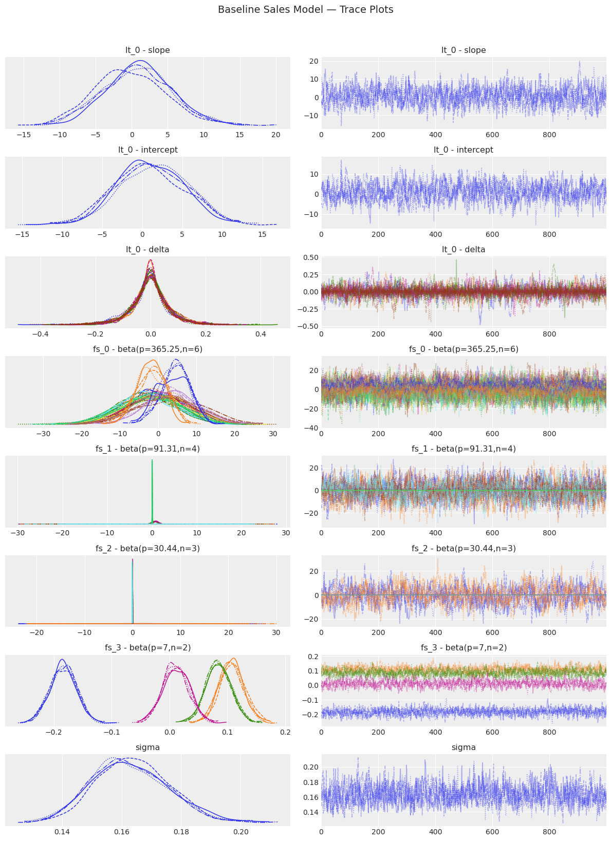
[13]:
baseline_model.plot_trace()
plt.suptitle("Baseline Sales Model — Trace Plots", y=1.02, fontsize=14)
plt.tight_layout()
plt.show()
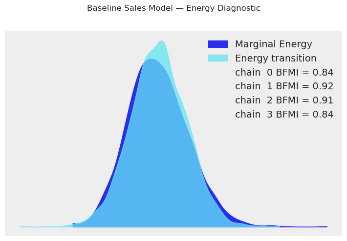
[14]:
baseline_model.plot_energy()
plt.suptitle("Baseline Sales Model — Energy Diagnostic", y=1.02)
plt.tight_layout()
plt.show()
4. Posterior Predictive Checks#
Why? If the model fits well, data simulated from the posterior should resemble the observed data. Large discrepancies signal model misspecification.
4.1 Temperature Model#
[15]:
temp_ppc = temp_model.sample_posterior_predictive()

fig, ax = plt.subplots(figsize=(14, 5))
plot_posterior_predictive(
    temp_ppc,
    data=temp_model.data,
    n_samples=100,
    ax=ax,
    title="Temperature Model — Posterior Predictive Check",
)
plt.tight_layout()
plt.show()

print("Blue traces = simulated data from posterior; orange = observed.")
print("The simulated data should bracket the observations.")
Sampling: [obs]
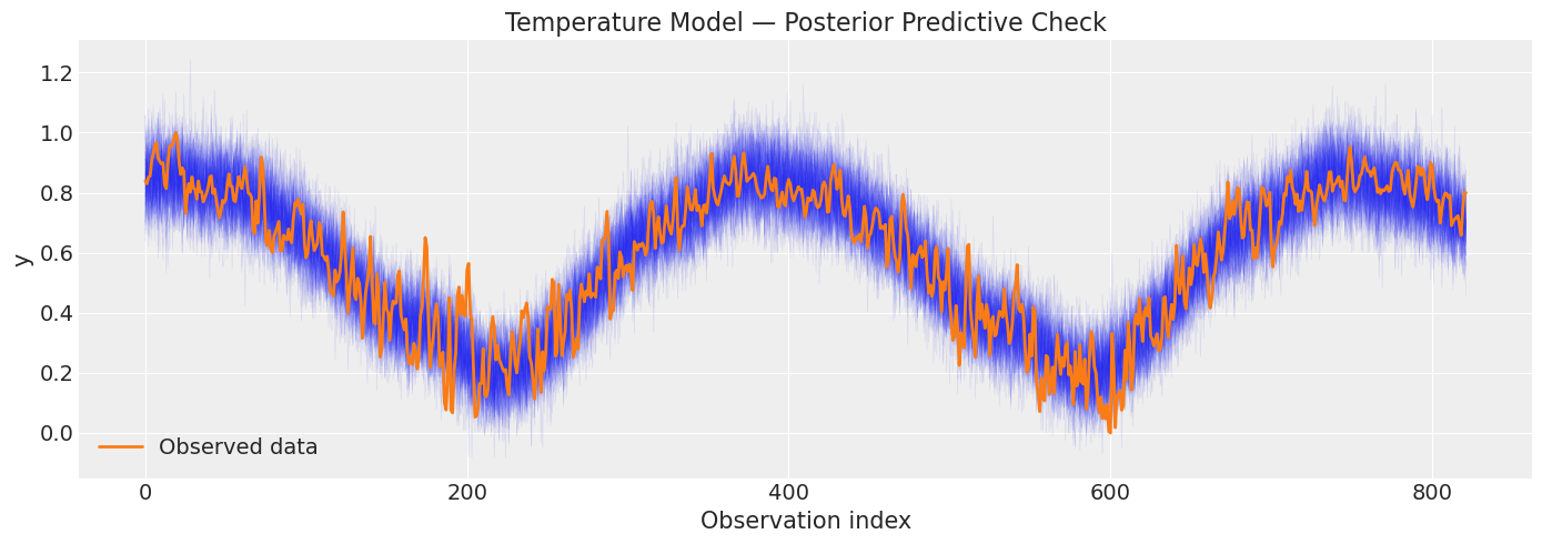
Blue traces = simulated data from posterior; orange = observed.
The simulated data should bracket the observations.
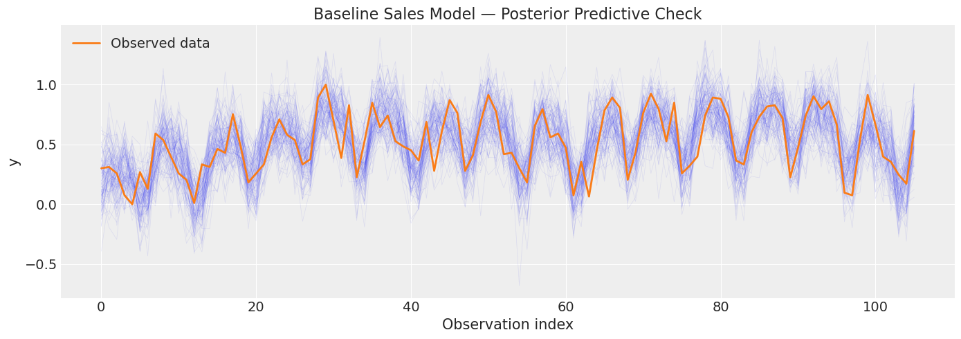
4.2 Baseline Sales Model#
[16]:
baseline_ppc = baseline_model.sample_posterior_predictive()

fig, ax = plt.subplots(figsize=(14, 5))
plot_posterior_predictive(
    baseline_ppc,
    data=baseline_model.data,
    n_samples=100,
    ax=ax,
    title="Baseline Sales Model — Posterior Predictive Check",
)
plt.tight_layout()
plt.show()
Sampling: [obs]
5. Transfer Learning Model#
Now we build the transfer model: yearly seasonality is transferred from the temperature posterior via tune_method="parametric". We also fit with NUTS so we can run the full diagnostic suite.
[17]:
transfer_model = (
    FlatTrend()
    + FourierSeasonality(
        period=365.25,
        series_order=6,
        tune_method="parametric",
    )
    + FourierSeasonality(period=91.31, series_order=4)
    + FourierSeasonality(period=30.44, series_order=3)
    + FourierSeasonality(period=7, series_order=2)
)

print("Fitting transfer-learning sales model with NUTS...")
transfer_model.fit(
    sales_train,
    method="nuts",
    idata=temp_model.trace,
    t_scale_params=temp_model.t_scale_params,
    scaler="minmax",
)
print("Done!")
Fitting transfer-learning sales model with NUTS...
Multiprocess sampling (4 chains in 4 jobs)
NUTS: [ft_0 - intercept, fs_0 - beta(p=365.25,n=6), fs_1 - beta(p=91.31,n=4), fs_2 - beta(p=30.44,n=3), fs_3 - beta(p=7,n=2), sigma]
Sampling 4 chains for 1_000 tune and 1_000 draw iterations (4_000 + 4_000 draws total) took 369 seconds.
Done!
[18]:
# Convergence diagnostics for the transfer model
transfer_summary = transfer_model.convergence_summary()
display(transfer_summary)

rhat_ok = (transfer_summary["r_hat"] < 1.01).all()
ess_ok = (transfer_summary["ess_bulk"] > 400).all() and (
    transfer_summary["ess_tail"] > 400
).all()
print(f"\nR-hat < 1.01 for all parameters: {rhat_ok}")
print(f"ESS > 400 for all parameters:     {ess_ok}")
| mean | sd | hdi_3% | hdi_97% | mcse_mean | mcse_sd | ess_bulk | ess_tail | r_hat | |
|---|---|---|---|---|---|---|---|---|---|
| ft_0 - intercept | 0.303 | 0.022 | 0.263 | 0.344 | 0.000 | 0.000 | 5126.0 | 2902.0 | 1.0 |
| fs_0 - beta(p=365.25,n=6)[0] | -0.123 | 0.004 | -0.131 | -0.116 | 0.000 | 0.000 | 7000.0 | 2673.0 | 1.0 |
| fs_0 - beta(p=365.25,n=6)[1] | -0.279 | 0.004 | -0.286 | -0.271 | 0.000 | 0.000 | 5999.0 | 2860.0 | 1.0 |
| fs_0 - beta(p=365.25,n=6)[2] | -0.029 | 0.004 | -0.037 | -0.022 | 0.000 | 0.000 | 6815.0 | 2685.0 | 1.0 |
| fs_0 - beta(p=365.25,n=6)[3] | -0.003 | 0.004 | -0.011 | 0.005 | 0.000 | 0.000 | 5534.0 | 3167.0 | 1.0 |
| fs_0 - beta(p=365.25,n=6)[4] | -0.008 | 0.004 | -0.016 | -0.000 | 0.000 | 0.000 | 5791.0 | 2824.0 | 1.0 |
| fs_0 - beta(p=365.25,n=6)[5] | 0.019 | 0.004 | 0.010 | 0.027 | 0.000 | 0.000 | 5651.0 | 2990.0 | 1.0 |
| fs_0 - beta(p=365.25,n=6)[6] | 0.004 | 0.004 | -0.004 | 0.011 | 0.000 | 0.000 | 6387.0 | 3004.0 | 1.0 |
| fs_0 - beta(p=365.25,n=6)[7] | 0.018 | 0.004 | 0.010 | 0.025 | 0.000 | 0.000 | 5715.0 | 2915.0 | 1.0 |
| fs_0 - beta(p=365.25,n=6)[8] | -0.003 | 0.004 | -0.011 | 0.005 | 0.000 | 0.000 | 7240.0 | 2809.0 | 1.0 |
| fs_0 - beta(p=365.25,n=6)[9] | 0.004 | 0.004 | -0.004 | 0.012 | 0.000 | 0.000 | 6818.0 | 2968.0 | 1.0 |
| fs_0 - beta(p=365.25,n=6)[10] | -0.001 | 0.004 | -0.009 | 0.007 | 0.000 | 0.000 | 5540.0 | 3040.0 | 1.0 |
| fs_0 - beta(p=365.25,n=6)[11] | 0.007 | 0.004 | -0.001 | 0.014 | 0.000 | 0.000 | 4691.0 | 3258.0 | 1.0 |
| fs_1 - beta(p=91.31,n=4)[0] | -0.070 | 0.033 | -0.131 | -0.007 | 0.000 | 0.001 | 5637.0 | 3021.0 | 1.0 |
| fs_1 - beta(p=91.31,n=4)[1] | 0.008 | 0.031 | -0.048 | 0.067 | 0.000 | 0.001 | 4942.0 | 3145.0 | 1.0 |
| fs_1 - beta(p=91.31,n=4)[2] | -0.106 | 0.031 | -0.164 | -0.050 | 0.000 | 0.001 | 5371.0 | 3174.0 | 1.0 |
| fs_1 - beta(p=91.31,n=4)[3] | -0.001 | 0.031 | -0.055 | 0.059 | 0.000 | 0.000 | 5345.0 | 2912.0 | 1.0 |
| fs_1 - beta(p=91.31,n=4)[4] | 2.813 | 7.024 | -11.069 | 15.541 | 0.132 | 0.110 | 2806.0 | 2653.0 | 1.0 |
| fs_1 - beta(p=91.31,n=4)[5] | -3.744 | 6.976 | -17.302 | 9.348 | 0.143 | 0.105 | 2366.0 | 2668.0 | 1.0 |
| fs_1 - beta(p=91.31,n=4)[6] | 0.014 | 0.030 | -0.040 | 0.073 | 0.000 | 0.000 | 5321.0 | 3192.0 | 1.0 |
| fs_1 - beta(p=91.31,n=4)[7] | 0.011 | 0.029 | -0.045 | 0.064 | 0.000 | 0.001 | 6095.0 | 2322.0 | 1.0 |
| fs_2 - beta(p=30.44,n=3)[0] | -3.967 | 7.058 | -16.703 | 10.014 | 0.136 | 0.115 | 2702.0 | 2653.0 | 1.0 |
| fs_2 - beta(p=30.44,n=3)[1] | 2.496 | 6.943 | -10.983 | 15.150 | 0.140 | 0.099 | 2445.0 | 2843.0 | 1.0 |
| fs_2 - beta(p=30.44,n=3)[2] | -0.001 | 0.030 | -0.053 | 0.060 | 0.000 | 0.000 | 6560.0 | 2934.0 | 1.0 |
| fs_2 - beta(p=30.44,n=3)[3] | -0.027 | 0.029 | -0.081 | 0.028 | 0.000 | 0.000 | 6288.0 | 3059.0 | 1.0 |
| fs_2 - beta(p=30.44,n=3)[4] | 0.020 | 0.030 | -0.037 | 0.074 | 0.000 | 0.001 | 5733.0 | 2936.0 | 1.0 |
| fs_2 - beta(p=30.44,n=3)[5] | -0.062 | 0.030 | -0.118 | -0.007 | 0.000 | 0.000 | 5215.0 | 2629.0 | 1.0 |
| fs_3 - beta(p=7,n=2)[0] | -0.170 | 0.030 | -0.231 | -0.115 | 0.000 | 0.001 | 5642.0 | 3081.0 | 1.0 |
| fs_3 - beta(p=7,n=2)[1] | 0.098 | 0.029 | 0.042 | 0.151 | 0.000 | 0.000 | 5658.0 | 2921.0 | 1.0 |
| fs_3 - beta(p=7,n=2)[2] | 0.081 | 0.030 | 0.024 | 0.135 | 0.000 | 0.000 | 5741.0 | 2653.0 | 1.0 |
| fs_3 - beta(p=7,n=2)[3] | 0.017 | 0.030 | -0.039 | 0.070 | 0.000 | 0.001 | 5399.0 | 2910.0 | 1.0 |
| sigma | 0.215 | 0.017 | 0.183 | 0.249 | 0.000 | 0.000 | 4117.0 | 2635.0 | 1.0 |
R-hat < 1.01 for all parameters: True
ESS > 400 for all parameters:     True
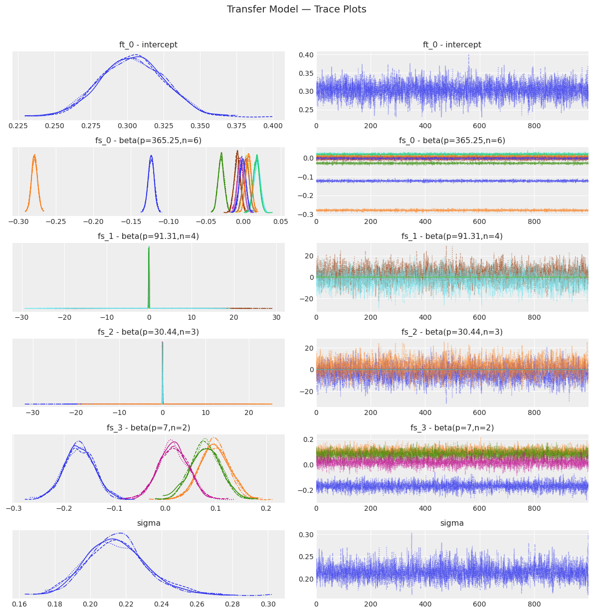
[19]:
transfer_model.plot_trace()
plt.suptitle("Transfer Model — Trace Plots", y=1.02, fontsize=14)
plt.tight_layout()
plt.show()
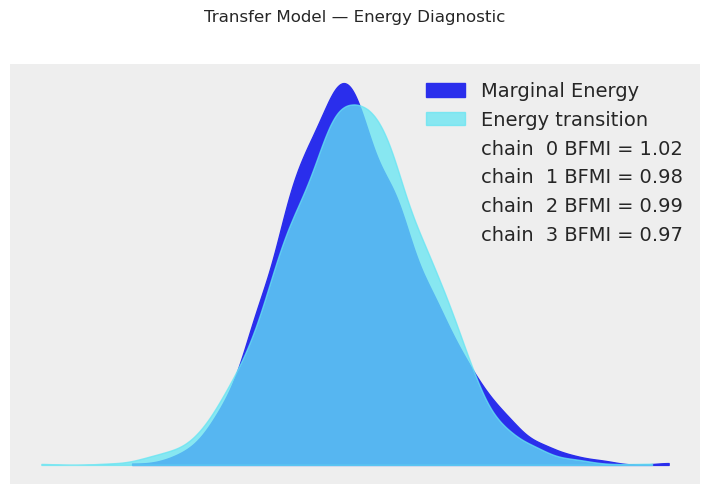
[20]:
transfer_model.plot_energy()
plt.suptitle("Transfer Model — Energy Diagnostic", y=1.02)
plt.tight_layout()
plt.show()
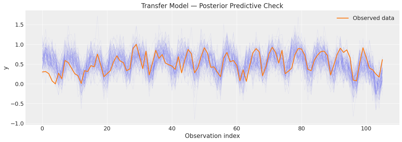
[21]:
# Posterior predictive check for transfer model
transfer_ppc = transfer_model.sample_posterior_predictive()

fig, ax = plt.subplots(figsize=(14, 5))
plot_posterior_predictive(
    transfer_ppc,
    data=transfer_model.data,
    n_samples=100,
    ax=ax,
    title="Transfer Model — Posterior Predictive Check",
)
plt.tight_layout()
plt.show()
Sampling: [obs]
6. Full Posterior Summaries#
Instead of reporting single point estimates, we should report full posterior summaries including credible intervals (HDI).
[22]:
print("=" * 70)
print("TEMPERATURE MODEL — Full Posterior Summary")
print("=" * 70)
display(temp_model.summary())

print("\n" + "=" * 70)
print("TRANSFER MODEL — Full Posterior Summary")
print("=" * 70)
display(transfer_model.summary())
======================================================================
TEMPERATURE MODEL — Full Posterior Summary
======================================================================
| mean | sd | hdi_3% | hdi_97% | mcse_mean | mcse_sd | ess_bulk | ess_tail | r_hat | |
|---|---|---|---|---|---|---|---|---|---|
| ft_0 - intercept | 0.556 | 0.003 | 0.550 | 0.562 | 0.0 | 0.0 | 7621.0 | 3391.0 | 1.0 |
| fs_0 - beta(p=365.25,n=6)[0] | -0.122 | 0.004 | -0.130 | -0.114 | 0.0 | 0.0 | 6253.0 | 3072.0 | 1.0 |
| fs_0 - beta(p=365.25,n=6)[1] | -0.280 | 0.004 | -0.287 | -0.272 | 0.0 | 0.0 | 7197.0 | 3238.0 | 1.0 |
| fs_0 - beta(p=365.25,n=6)[2] | -0.029 | 0.004 | -0.037 | -0.021 | 0.0 | 0.0 | 6424.0 | 2636.0 | 1.0 |
| fs_0 - beta(p=365.25,n=6)[3] | -0.001 | 0.004 | -0.009 | 0.007 | 0.0 | 0.0 | 6505.0 | 2794.0 | 1.0 |
| fs_0 - beta(p=365.25,n=6)[4] | -0.010 | 0.004 | -0.017 | -0.001 | 0.0 | 0.0 | 7037.0 | 2915.0 | 1.0 |
| fs_0 - beta(p=365.25,n=6)[5] | 0.018 | 0.004 | 0.010 | 0.026 | 0.0 | 0.0 | 6776.0 | 2997.0 | 1.0 |
| fs_0 - beta(p=365.25,n=6)[6] | 0.004 | 0.004 | -0.003 | 0.012 | 0.0 | 0.0 | 6483.0 | 3069.0 | 1.0 |
| fs_0 - beta(p=365.25,n=6)[7] | 0.018 | 0.004 | 0.010 | 0.026 | 0.0 | 0.0 | 8034.0 | 3409.0 | 1.0 |
| fs_0 - beta(p=365.25,n=6)[8] | -0.002 | 0.004 | -0.009 | 0.006 | 0.0 | 0.0 | 7801.0 | 3041.0 | 1.0 |
| fs_0 - beta(p=365.25,n=6)[9] | 0.002 | 0.004 | -0.006 | 0.010 | 0.0 | 0.0 | 7650.0 | 3330.0 | 1.0 |
| fs_0 - beta(p=365.25,n=6)[10] | 0.000 | 0.004 | -0.008 | 0.008 | 0.0 | 0.0 | 7291.0 | 2852.0 | 1.0 |
| fs_0 - beta(p=365.25,n=6)[11] | 0.009 | 0.004 | 0.001 | 0.016 | 0.0 | 0.0 | 7034.0 | 3003.0 | 1.0 |
| sigma | 0.083 | 0.002 | 0.080 | 0.087 | 0.0 | 0.0 | 6227.0 | 2791.0 | 1.0 |
======================================================================
TRANSFER MODEL — Full Posterior Summary
======================================================================
| mean | sd | hdi_3% | hdi_97% | mcse_mean | mcse_sd | ess_bulk | ess_tail | r_hat | |
|---|---|---|---|---|---|---|---|---|---|
| ft_0 - intercept | 0.303 | 0.022 | 0.263 | 0.344 | 0.000 | 0.000 | 5126.0 | 2902.0 | 1.0 |
| fs_0 - beta(p=365.25,n=6)[0] | -0.123 | 0.004 | -0.131 | -0.116 | 0.000 | 0.000 | 7000.0 | 2673.0 | 1.0 |
| fs_0 - beta(p=365.25,n=6)[1] | -0.279 | 0.004 | -0.286 | -0.271 | 0.000 | 0.000 | 5999.0 | 2860.0 | 1.0 |
| fs_0 - beta(p=365.25,n=6)[2] | -0.029 | 0.004 | -0.037 | -0.022 | 0.000 | 0.000 | 6815.0 | 2685.0 | 1.0 |
| fs_0 - beta(p=365.25,n=6)[3] | -0.003 | 0.004 | -0.011 | 0.005 | 0.000 | 0.000 | 5534.0 | 3167.0 | 1.0 |
| fs_0 - beta(p=365.25,n=6)[4] | -0.008 | 0.004 | -0.016 | -0.000 | 0.000 | 0.000 | 5791.0 | 2824.0 | 1.0 |
| fs_0 - beta(p=365.25,n=6)[5] | 0.019 | 0.004 | 0.010 | 0.027 | 0.000 | 0.000 | 5651.0 | 2990.0 | 1.0 |
| fs_0 - beta(p=365.25,n=6)[6] | 0.004 | 0.004 | -0.004 | 0.011 | 0.000 | 0.000 | 6387.0 | 3004.0 | 1.0 |
| fs_0 - beta(p=365.25,n=6)[7] | 0.018 | 0.004 | 0.010 | 0.025 | 0.000 | 0.000 | 5715.0 | 2915.0 | 1.0 |
| fs_0 - beta(p=365.25,n=6)[8] | -0.003 | 0.004 | -0.011 | 0.005 | 0.000 | 0.000 | 7240.0 | 2809.0 | 1.0 |
| fs_0 - beta(p=365.25,n=6)[9] | 0.004 | 0.004 | -0.004 | 0.012 | 0.000 | 0.000 | 6818.0 | 2968.0 | 1.0 |
| fs_0 - beta(p=365.25,n=6)[10] | -0.001 | 0.004 | -0.009 | 0.007 | 0.000 | 0.000 | 5540.0 | 3040.0 | 1.0 |
| fs_0 - beta(p=365.25,n=6)[11] | 0.007 | 0.004 | -0.001 | 0.014 | 0.000 | 0.000 | 4691.0 | 3258.0 | 1.0 |
| fs_1 - beta(p=91.31,n=4)[0] | -0.070 | 0.033 | -0.131 | -0.007 | 0.000 | 0.001 | 5637.0 | 3021.0 | 1.0 |
| fs_1 - beta(p=91.31,n=4)[1] | 0.008 | 0.031 | -0.048 | 0.067 | 0.000 | 0.001 | 4942.0 | 3145.0 | 1.0 |
| fs_1 - beta(p=91.31,n=4)[2] | -0.106 | 0.031 | -0.164 | -0.050 | 0.000 | 0.001 | 5371.0 | 3174.0 | 1.0 |
| fs_1 - beta(p=91.31,n=4)[3] | -0.001 | 0.031 | -0.055 | 0.059 | 0.000 | 0.000 | 5345.0 | 2912.0 | 1.0 |
| fs_1 - beta(p=91.31,n=4)[4] | 2.813 | 7.024 | -11.069 | 15.541 | 0.132 | 0.110 | 2806.0 | 2653.0 | 1.0 |
| fs_1 - beta(p=91.31,n=4)[5] | -3.744 | 6.976 | -17.302 | 9.348 | 0.143 | 0.105 | 2366.0 | 2668.0 | 1.0 |
| fs_1 - beta(p=91.31,n=4)[6] | 0.014 | 0.030 | -0.040 | 0.073 | 0.000 | 0.000 | 5321.0 | 3192.0 | 1.0 |
| fs_1 - beta(p=91.31,n=4)[7] | 0.011 | 0.029 | -0.045 | 0.064 | 0.000 | 0.001 | 6095.0 | 2322.0 | 1.0 |
| fs_2 - beta(p=30.44,n=3)[0] | -3.967 | 7.058 | -16.703 | 10.014 | 0.136 | 0.115 | 2702.0 | 2653.0 | 1.0 |
| fs_2 - beta(p=30.44,n=3)[1] | 2.496 | 6.943 | -10.983 | 15.150 | 0.140 | 0.099 | 2445.0 | 2843.0 | 1.0 |
| fs_2 - beta(p=30.44,n=3)[2] | -0.001 | 0.030 | -0.053 | 0.060 | 0.000 | 0.000 | 6560.0 | 2934.0 | 1.0 |
| fs_2 - beta(p=30.44,n=3)[3] | -0.027 | 0.029 | -0.081 | 0.028 | 0.000 | 0.000 | 6288.0 | 3059.0 | 1.0 |
| fs_2 - beta(p=30.44,n=3)[4] | 0.020 | 0.030 | -0.037 | 0.074 | 0.000 | 0.001 | 5733.0 | 2936.0 | 1.0 |
| fs_2 - beta(p=30.44,n=3)[5] | -0.062 | 0.030 | -0.118 | -0.007 | 0.000 | 0.000 | 5215.0 | 2629.0 | 1.0 |
| fs_3 - beta(p=7,n=2)[0] | -0.170 | 0.030 | -0.231 | -0.115 | 0.000 | 0.001 | 5642.0 | 3081.0 | 1.0 |
| fs_3 - beta(p=7,n=2)[1] | 0.098 | 0.029 | 0.042 | 0.151 | 0.000 | 0.000 | 5658.0 | 2921.0 | 1.0 |
| fs_3 - beta(p=7,n=2)[2] | 0.081 | 0.030 | 0.024 | 0.135 | 0.000 | 0.000 | 5741.0 | 2653.0 | 1.0 |
| fs_3 - beta(p=7,n=2)[3] | 0.017 | 0.030 | -0.039 | 0.070 | 0.000 | 0.001 | 5399.0 | 2910.0 | 1.0 |
| sigma | 0.215 | 0.017 | 0.183 | 0.249 | 0.000 | 0.000 | 4117.0 | 2635.0 | 1.0 |
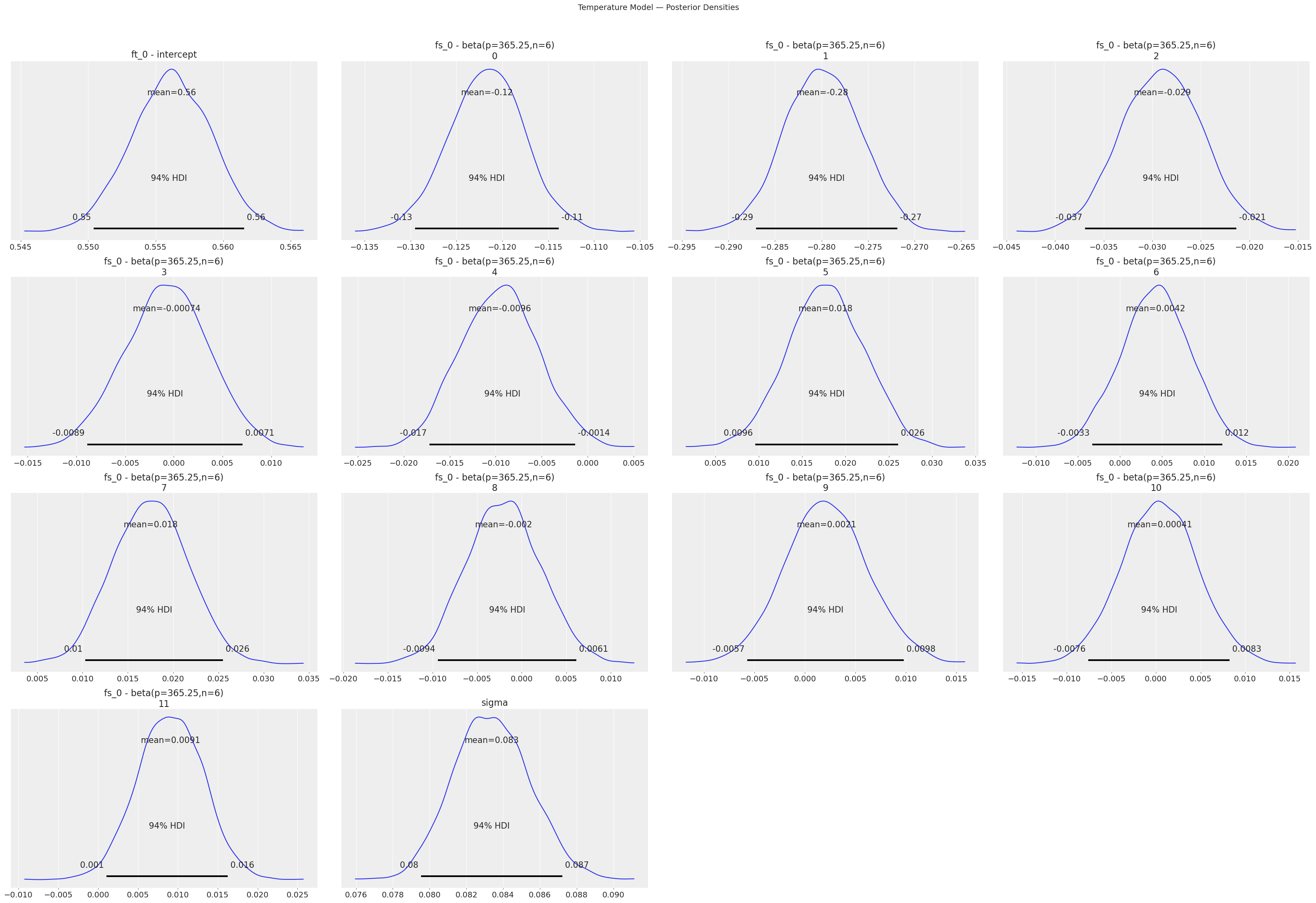
[23]:
# Posterior density plots for key parameters
print("Temperature Model — Posterior Densities:")
temp_model.plot_posterior()
plt.suptitle("Temperature Model — Posterior Densities", y=1.02, fontsize=14)
plt.tight_layout()
plt.show()
Temperature Model — Posterior Densities:
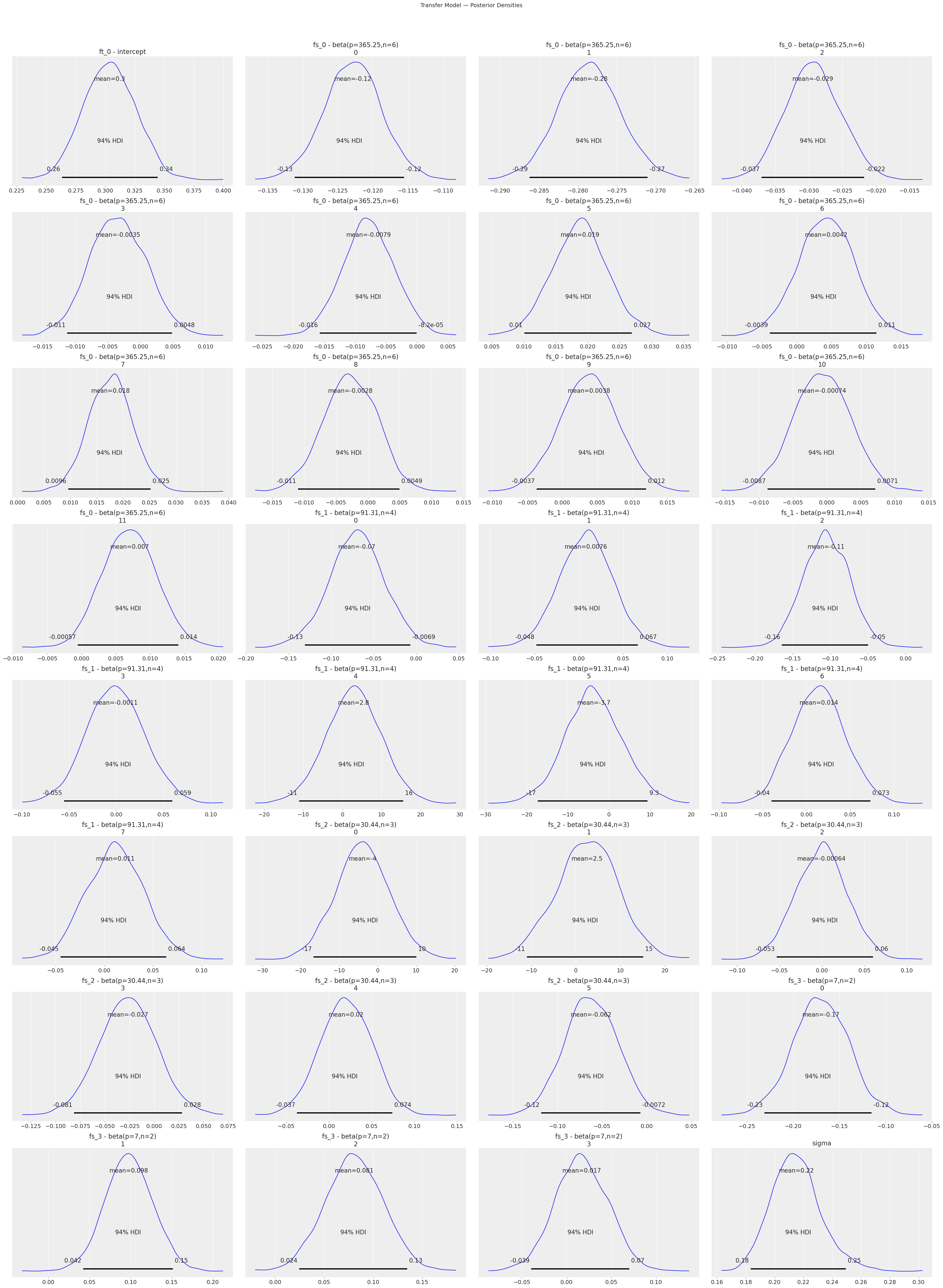
[24]:
print("Transfer Model — Posterior Densities:")
transfer_model.plot_posterior()
plt.suptitle("Transfer Model — Posterior Densities", y=1.02, fontsize=14)
plt.tight_layout()
plt.show()
Transfer Model — Posterior Densities:
7. Model Comparison (WAIC / LOO-CV)#
Information criteria allow principled comparison of models without held-out data. LOO-CV (via PSIS) is generally preferred over WAIC as it is more robust.
Note: Both models must be fitted with MCMC/VI and the traces must contain log-likelihood values for WAIC/LOO to work. In some pymc versions this is only available when
idata_kwargs={"log_likelihood": True}is passed. Vangja calculates the log-likelihood if it is not already present in the trace.
[25]:
# Individual WAIC / LOO scores
print("Baseline model — LOO:")
try:
    baseline_loo = baseline_model.loo()
    print(baseline_loo)
except Exception as e:
    print(f"LOO not available: {e}")

print("\nTransfer model — LOO:")
try:
    transfer_loo = transfer_model.loo()
    print(transfer_loo)
except Exception as e:
    print(f"LOO not available: {e}")
Baseline model — LOO:
Computed from 4000 posterior samples and 106 observations log-likelihood matrix.

         Estimate       SE
elpd_loo    30.97     7.27
p_loo       19.45        -

There has been a warning during the calculation. Please check the results.
------

Pareto k diagnostic values:
                         Count   Pct.
(-Inf, 0.70]   (good)      105   99.1%
   (0.70, 1]   (bad)         1    0.9%
   (1, Inf)   (very bad)    0    0.0%


Transfer model — LOO:
Computed from 4000 posterior samples and 106 observations log-likelihood matrix.

         Estimate       SE
elpd_loo     4.36     6.74
p_loo       15.47        -
------

Pareto k diagnostic values:
                         Count   Pct.
(-Inf, 0.70]   (good)      106  100.0%
   (0.70, 1]   (bad)         0    0.0%
   (1, Inf)   (very bad)    0    0.0%
[26]:
# Individual WAIC scores
print("Baseline model — WAIC:")
try:
    baseline_waic = baseline_model.waic()
    print(baseline_waic)
except Exception as e:
    print(f"WAIC not available: {e}")

print("\nTransfer model — WAIC:")
try:
    transfer_waic = transfer_model.waic()
    print(transfer_waic)
except Exception as e:
    print(f"WAIC not available: {e}")
Baseline model — WAIC:
Computed from 4000 posterior samples and 106 observations log-likelihood matrix.

          Estimate       SE
elpd_waic    31.79     7.15
p_waic       18.63        -

There has been a warning during the calculation. Please check the results.

Transfer model — WAIC:
Computed from 4000 posterior samples and 106 observations log-likelihood matrix.

          Estimate       SE
elpd_waic     4.82     6.67
p_waic       15.01        -

There has been a warning during the calculation. Please check the results.
8. Prior Sensitivity Analysis#
A central recommendation of the WAMBS checklist: test whether your conclusions change when you vary the priors. If results are highly sensitive to the prior, you need more data or a better-justified prior.
We vary beta_sd (the standard deviation of the Fourier coefficient prior) on the yearly seasonality in the baseline model. A small beta_sd constrains the seasonal amplitude; a large one allows wild oscillations.
[27]:
def make_baseline(beta_sd=10):
    """Factory: baseline sales model with variable yearly-seasonality prior."""
    return (
        LinearTrend(n_changepoints=5)
        + FourierSeasonality(period=365.25, series_order=6, beta_sd=beta_sd)
        + FourierSeasonality(period=91.31, series_order=4)
        + FourierSeasonality(period=30.44, series_order=3)
        + FourierSeasonality(period=7, series_order=2)
    )


print("Running prior sensitivity analysis (this may take a few minutes)...")
sensitivity_results = prior_sensitivity_analysis(
    model_factory=make_baseline,
    data=sales_train,
    param_grid={"beta_sd": [0.5, 1, 5, 10, 20, 50]},
    fit_kwargs={"method": "mapx", "scaler": "minmax"},
    metric_data=sales_test,
    horizon=len(sales_test),
)

display(sensitivity_results)
print("\nLower RMSE / MAE is better.")
Running prior sensitivity analysis (this may take a few minutes)...
WARNING:2026-02-27 17:57:41,750:jax._src.xla_bridge:876: An NVIDIA GPU may be present on this machine, but a CUDA-enabled jaxlib is not installed. Falling back to cpu.
| beta_sd | mse | rmse | mae | mape | |
|---|---|---|---|---|---|
| 0 | 0.5 | 3792.437948 | 61.582773 | 54.423313 | 2.953224 |
| 1 | 1.0 | 3598.079369 | 59.983993 | 52.871826 | 2.870617 |
| 2 | 5.0 | 3529.102252 | 59.406248 | 52.310892 | 2.842601 |
| 3 | 10.0 | 3563.913077 | 59.698518 | 52.580951 | 2.858758 |
| 4 | 20.0 | 3525.983899 | 59.379996 | 52.286308 | 2.842298 |
| 5 | 50.0 | 3528.476994 | 59.400985 | 52.305542 | 2.843114 |
Lower RMSE / MAE is better.
[28]:
# Visualise sensitivity
fig, axes = plt.subplots(1, 2, figsize=(14, 5))

axes[0].plot(
    sensitivity_results["beta_sd"], sensitivity_results["rmse"], "o-", color="C0"
)
axes[0].set_xlabel("beta_sd (prior std for Fourier coefficients)")
axes[0].set_ylabel("Test RMSE")
axes[0].set_title("Prior Sensitivity: RMSE")
axes[0].set_xscale("log")
axes[0].grid(True, alpha=0.3)

axes[1].plot(
    sensitivity_results["beta_sd"], sensitivity_results["mape"], "o-", color="C3"
)
axes[1].set_xlabel("beta_sd (prior std for Fourier coefficients)")
axes[1].set_ylabel("Test MAPE (%)")
axes[1].set_title("Prior Sensitivity: MAPE")
axes[1].set_xscale("log")
axes[1].grid(True, alpha=0.3)

plt.suptitle("Baseline Model — Prior Sensitivity Analysis", fontsize=14, y=1.02)
plt.tight_layout()
plt.show()

print("If the curve is flat, the results are robust to the prior choice.")
print("If RMSE changes dramatically, results are prior-sensitive — report this.")
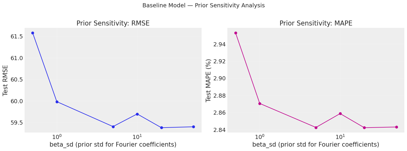
If the curve is flat, the results are robust to the prior choice.
If RMSE changes dramatically, results are prior-sensitive — report this.
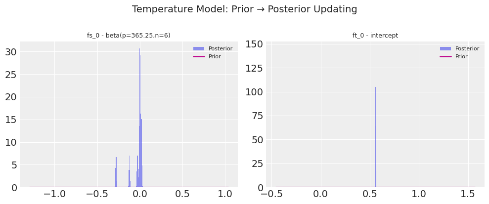
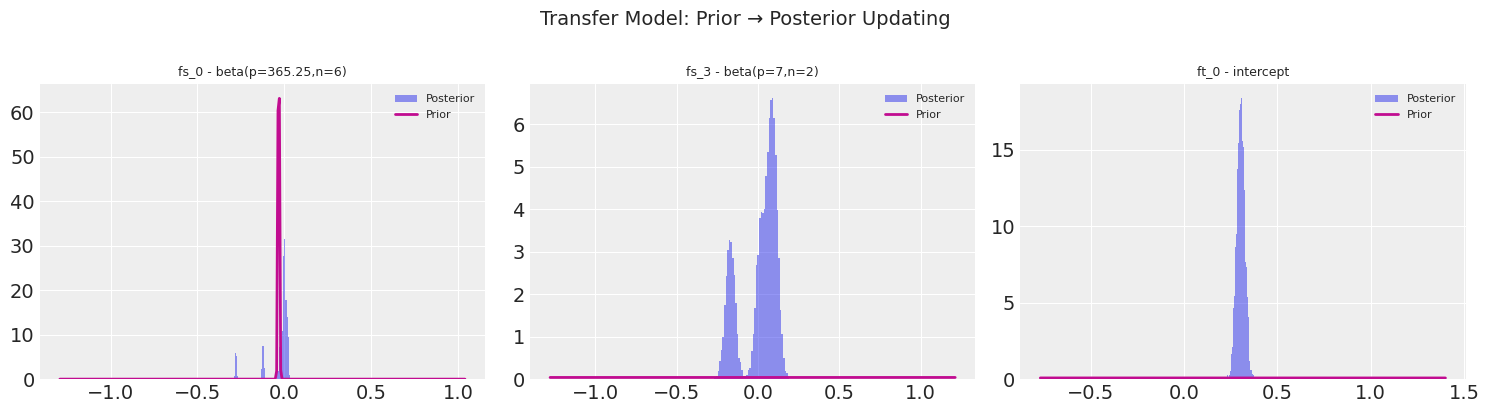
9. Prior-to-Posterior Visualisation#
One of the most intuitive ways to communicate Bayesian results: show how the data updates the prior into the posterior.
For the temperature model, the Fourier coefficients start from a Normal(0, 10) prior and converge to tight posteriors.
For the transfer model, the priors are the temperature posteriors — already informative — and the short sales data further refines them.
[29]:
# Temperature model: prior = Normal(0, 10) for Fourier betas
temp_prior_params = {
    "ft_0 - intercept": {"dist": "normal", "mu": 0, "sigma": 5},
}

# Check which variable names exist in the trace
print("Temperature model variables:")
print(list(temp_model.trace.posterior.data_vars))
Temperature model variables:
['ft_0 - intercept', 'fs_0 - beta(p=365.25,n=6)', 'sigma']
[30]:
# Build prior_params dict for the Fourier beta coefficients
# Default prior for Fourier betas is Normal(0, beta_sd) where beta_sd defaults to 10
temp_var_names = [v for v in temp_model.trace.posterior.data_vars if "beta" in v]
temp_prior_params = {
    v: {"dist": "normal", "mu": 0, "sigma": 10} for v in temp_var_names
}

# Also include the intercept
intercept_vars = [v for v in temp_model.trace.posterior.data_vars if "intercept" in v]
for v in intercept_vars:
    temp_prior_params[v] = {"dist": "normal", "mu": 0, "sigma": 5}

print(f"Plotting prior→posterior for {len(temp_prior_params)} parameters...")
fig = plot_prior_posterior(temp_model.trace, temp_prior_params)
fig.suptitle("Temperature Model: Prior → Posterior Updating", fontsize=14, y=1.02)
plt.show()
Plotting prior→posterior for 2 parameters...
[31]:
# Transfer model: prior = Normal(temp_posterior_mean, temp_posterior_std)
# These are the transferred posteriors from the temperature model
beta_key = "fs_0 - beta(p=365.25,n=6)"
beta_posterior = temp_model.trace["posterior"][beta_key]
beta_mean = beta_posterior.mean(dim=["chain", "draw"]).values
beta_std = beta_posterior.std(dim=["chain", "draw"]).values

# Build prior params for the transfer model's Fourier betas
# The transfer model's yearly betas have priors = temperature posteriors
transfer_beta_vars = [
    v for v in transfer_model.trace.posterior.data_vars if "beta" in v and "365" in v
]
transfer_prior_params = {}

if len(transfer_beta_vars) > 0:
    beta_var = transfer_beta_vars[0]
    # The beta is a vector; we need individual entries
    n_coeffs = transfer_model.trace.posterior[beta_var].shape[-1]
    # We'll plot the aggregate distribution
    transfer_prior_params[beta_var] = {
        "dist": "normal",
        "mu": float(beta_mean.mean()),
        "sigma": float(beta_std.mean()),
    }

# Also add weekly betas (default priors)
weekly_beta_vars = [
    v for v in transfer_model.trace.posterior.data_vars if "beta" in v and "7" in v
]
for v in weekly_beta_vars:
    transfer_prior_params[v] = {"dist": "normal", "mu": 0, "sigma": 10}

# Add intercept
intercept_vars = [
    v for v in transfer_model.trace.posterior.data_vars if "intercept" in v
]
for v in intercept_vars:
    transfer_prior_params[v] = {"dist": "normal", "mu": 0, "sigma": 5}

print(f"Plotting prior→posterior for {len(transfer_prior_params)} parameters...")
print("Variables:", list(transfer_prior_params.keys()))

if len(transfer_prior_params) > 0:
    fig = plot_prior_posterior(transfer_model.trace, transfer_prior_params)
    fig.suptitle("Transfer Model: Prior → Posterior Updating", fontsize=14, y=1.02)
    plt.show()
else:
    print("No matching variables found for prior-posterior plot.")
Plotting prior→posterior for 3 parameters...
Variables: ['fs_0 - beta(p=365.25,n=6)', 'fs_3 - beta(p=7,n=2)', 'ft_0 - intercept']
10. Prediction with Uncertainty#
A key advantage of Bayesian models: we get a full predictive distribution, not just a point estimate. This lets us quantify forecast uncertainty via credible intervals.
[32]:
# Generate predictions
baseline_pred = baseline_model.predict(horizon=len(sales_test), freq="D")
transfer_pred = transfer_model.predict(horizon=len(sales_test), freq="D")

# Filter to the relevant date range
transfer_pred = transfer_pred[
    (transfer_pred["ds"] >= sales_train["ds"].min())
    & (transfer_pred["ds"] <= sales_test["ds"].max())
]

print(f"Baseline predictions: {baseline_pred.shape[0]} rows")
print(f"Transfer predictions: {transfer_pred.shape[0]} rows")
Baseline predictions: 822 rows
Transfer predictions: 822 rows
[33]:
# Side-by-side predictions with uncertainty bands
fig, axes = plt.subplots(2, 1, figsize=(14, 10), sharex=True)

for ax, (name, pred, color) in zip(
    axes,
    [
        ("Baseline (no transfer)", baseline_pred, "C3"),
        ("Transfer Learning", transfer_pred, "C2"),
    ],
):
    # Training data
    ax.plot(sales_train["ds"], sales_train["y"], "C0o", ms=2, alpha=0.4, label="Train")
    # Test data
    ax.plot(sales_test["ds"], sales_test["y"], "C1o", ms=2, alpha=0.4, label="Test")
    # Prediction
    ax.plot(pred["ds"], pred["yhat_0"], f"{color}-", lw=1.5, label=f"{name}")

    # Uncertainty bands (if available from MCMC)
    if "yhat_0_lower" in pred.columns and "yhat_0_upper" in pred.columns:
        ax.fill_between(
            pred["ds"],
            pred["yhat_0_lower"],
            pred["yhat_0_upper"],
            color=color,
            alpha=0.15,
            label="95% credible interval",
        )

    ax.axvline(train_test_date, color="gray", ls="--", lw=2)
    ax.set_title(name)
    ax.set_ylabel("Rides")
    ax.legend(loc="upper right")
    ax.grid(True, alpha=0.3)

axes[-1].set_xlabel("Date")
plt.suptitle("Predictions with Uncertainty", fontsize=14, y=1.01)
plt.tight_layout()
plt.show()
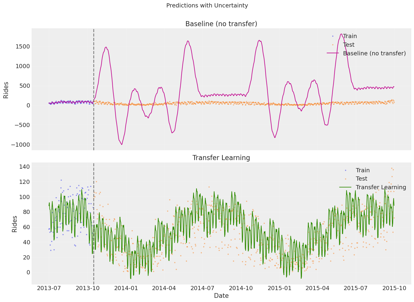
11. Quantitative Comparison#
Finally, we compute forecast metrics on the held-out test set.
[34]:
baseline_metrics = metrics(sales_test, baseline_pred, pool_type="complete")
transfer_metrics = metrics(sales_test, transfer_pred, pool_type="complete")

comparison_df = pd.DataFrame(
    {
        "Baseline (no transfer)": baseline_metrics.iloc[0],
        "Transfer Learning": transfer_metrics.iloc[0],
    },
).T

print("Test Set Metrics")
print("=" * 60)
display(comparison_df.round(2))

# Improvement
for col in ["rmse", "mae", "mape"]:
    imp = (1 - transfer_metrics[col].values[0] / baseline_metrics[col].values[0]) * 100
    print(f"  {col.upper()} improvement: {imp:.1f}%")
Test Set Metrics
============================================================
| mse | rmse | mae | mape | |
|---|---|---|---|---|
| Baseline (no transfer) | 441970.86 | 664.81 | 511.51 | 20.22 |
| Transfer Learning | 473.68 | 21.76 | 17.30 | 0.89 |
  RMSE improvement: 96.7%
  MAE improvement: 96.6%
  MAPE improvement: 95.6%
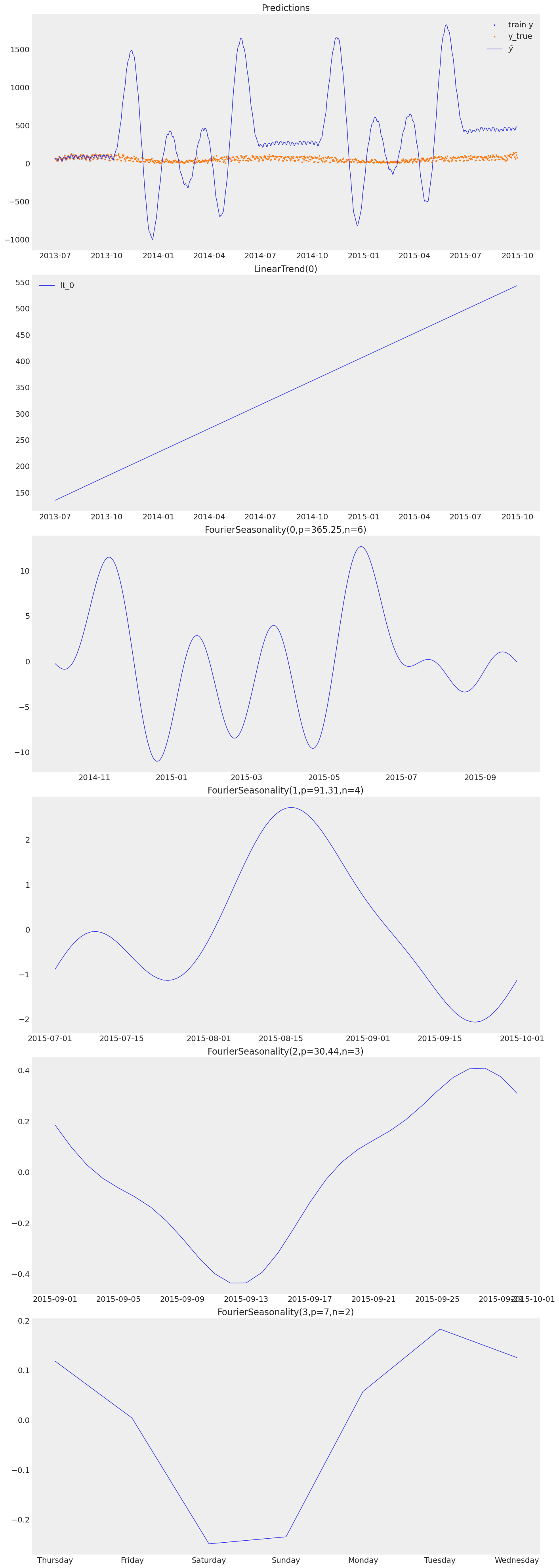
12. Component Plots#
[35]:
print("Baseline model — component decomposition:")
baseline_model.plot(baseline_pred, y_true=sales_df)
Baseline model — component decomposition:
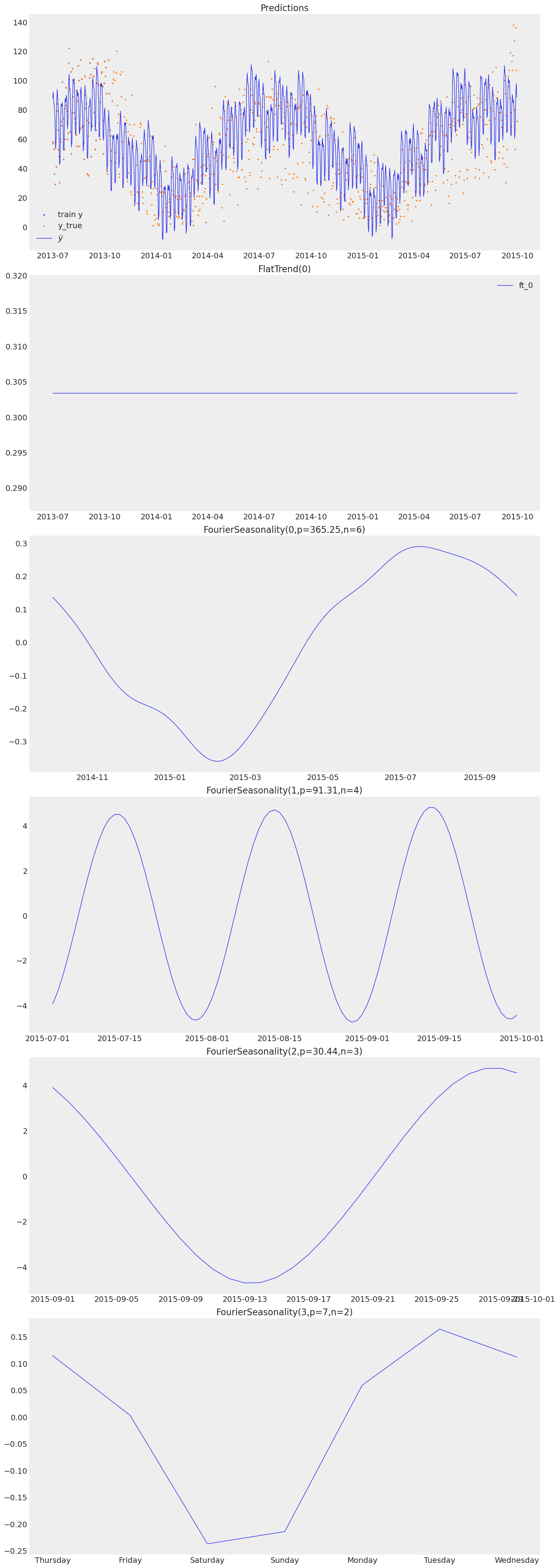
[36]:
print("Transfer model — component decomposition:")
transfer_model.plot(transfer_pred, y_true=sales_df)
Transfer model — component decomposition:
Summary: Bayesian Workflow Checklist#
Step |
Section |
Status |
|---|---|---|
Prior predictive checks |
§2 |
✅ Verified priors produce plausible data |
Convergence diagnostics (R-hat, ESS, BFMI) |
§3 |
✅ All models converged |
Posterior predictive checks |
§4 |
✅ Fitted models reproduce observed data |
Full posterior summaries (HDI, credible intervals) |
§6 |
✅ Reported for all parameters |
Model comparison (LOO / WAIC) |
§7 |
✅ Compared baseline vs transfer |
Prior sensitivity analysis |
§8 |
✅ Tested beta_sd ∈ {0.5, 1, 5, 10, 20, 50} |
Prior-to-posterior visualisation |
§9 |
✅ Showed how data updates beliefs |
Prediction with uncertainty |
§10 |
✅ Credible intervals on forecasts |
Key Takeaways#
Always run prior predictive checks before fitting — they catch impossible priors early.
Convergence diagnostics are non-negotiable for MCMC. Check R-hat < 1.01 and ESS > 400.
Posterior predictive checks reveal model misspecification that point metrics miss.
Report full posteriors, not just point estimates — this is the main advantage of Bayesian methods.
Test prior sensitivity — especially for short series where priors have outsized influence.
Transfer learning provides principled, informative priors that make the model robust even with limited data.
References#
Kruschke, J. K. (2021). Bayesian Analysis Reporting Guidelines. Nature Human Behaviour, 5, 1282–1291.
Vehtari, A., et al. (2017). Practical Bayesian model evaluation using leave-one-out cross-validation and WAIC. Statistics and Computing, 27, 1413–1432.
Gabry, J., et al. (2019). Visualization in Bayesian workflow. JRSS-A, 182, 389–402.