Chapter 07: Transfer Learning from Long Time Series#
Forecasting short time series is notoriously difficult. With only a few weeks or months of data, traditional methods struggle to capture long-term patterns like yearly seasonality. Yet in many business contexts, we know such patterns exist — we just haven’t observed them yet.
This chapter demonstrates how to use transfer learning to overcome this limitation. The key insight: if we have a long time series that shares seasonal patterns with our short target series, we can:
Fit a model to the long series to learn its seasonal structure
Transfer the learned posteriors as priors to the short series model
This approach was inspired by:
Modeling Short Time Series with Prior Knowledge by Tim Radtke
Modeling Short Time Series with Prior Knowledge in PyMC by Juan Orduz
Vangja was partially inspired by these two blog posts and implements parametric transfer learning as a core feature.
The Scenario#
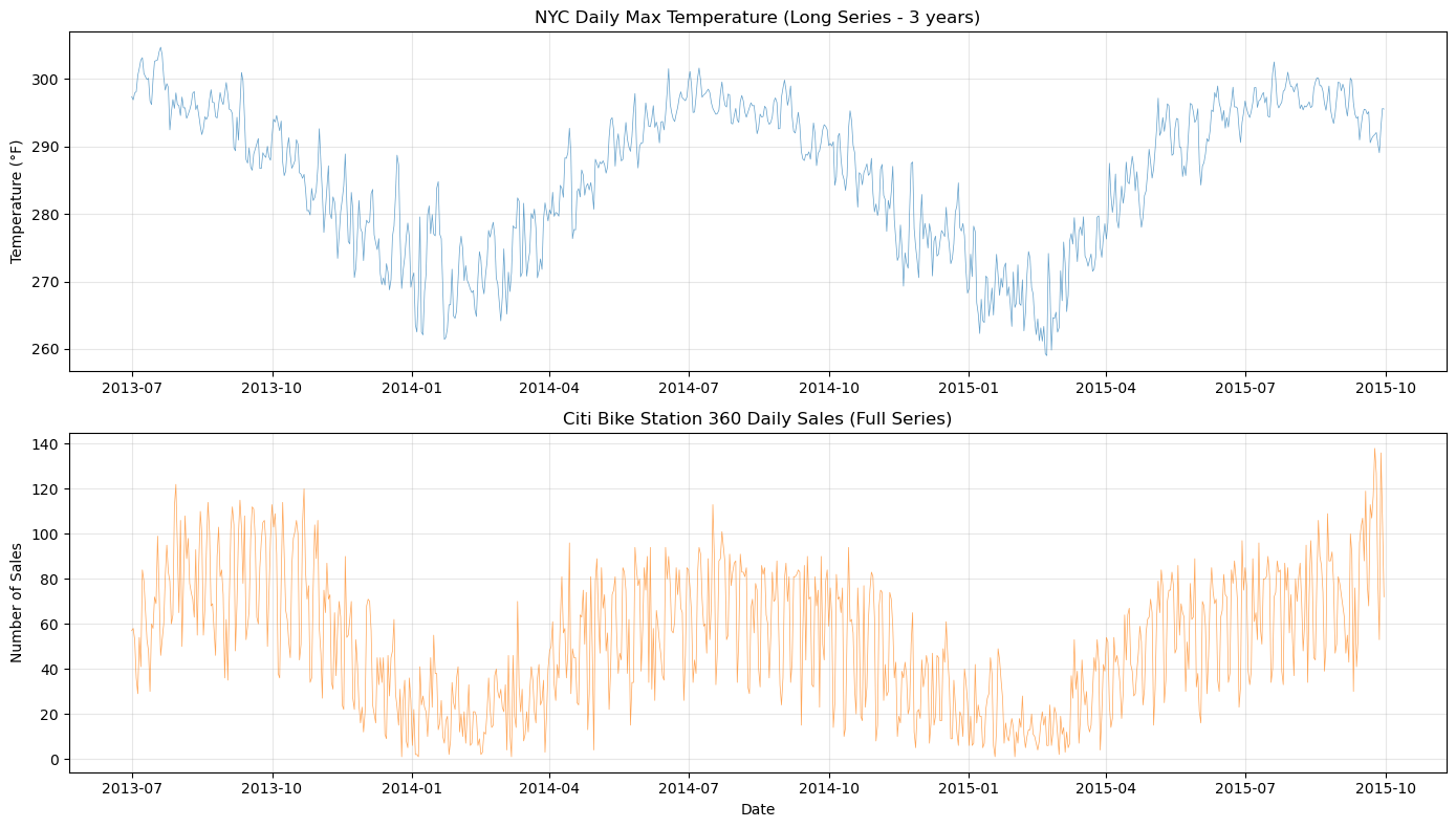
We have daily bike sales data from a Citi Bike station in NYC, but only ~3 months of history (July–October 2013). We need to forecast sales for the next year, including through winter and back to summer.
The challenge: with only summer/fall data, how can we capture the yearly seasonality pattern where demand drops significantly in winter?
The solution: New York City temperature has a strong yearly pattern that correlates with bike demand. Even though we can’t use temperature directly as a predictor (we’d need future forecasts), we can learn the shape of yearly seasonality from historical temperature data and transfer it to our sales model.
Differences from the Original Blog Posts#
The original implementations use a more complex model structure:
A negative binomial likelihood with autoregressive (AR) components on the latent mean
A damped dynamic model: \(\mu_t = (1-\delta-\eta)\lambda_t + \delta\mu_{t-1} + \eta y_{t-1}\)
Vangja uses a simpler Prophet-like approach:
A piecewise
LinearTrendcomponent instead of AR dynamicsGaussian likelihood
Transfer learning via the
tune_method="parametric"parameter onFourierSeasonality
Despite these differences, the core insight — transferring learned seasonality via Bayesian priors — works remarkably well.
Setup and Imports#
[1]:
import warnings

warnings.filterwarnings("ignore")
[2]:
import matplotlib.pyplot as plt
import numpy as np
import pandas as pd

from vangja import FlatTrend, FourierSeasonality, LinearTrend
from vangja.datasets import load_citi_bike_sales, load_nyc_temperature
from vangja.utils import metrics

print("Imports successful!")
Imports successful!
Load and Explore the Data#
We load two datasets:
Temperature data: ~5 years of daily max temperatures for NYC (our “long” series)
Bike sales data: ~16 months of daily bike rides from Citi Bike station 360 (we’ll use only ~3 months for training)
[3]:
# Load the datasets
temp_df = load_nyc_temperature()
sales_df = load_citi_bike_sales()

# The original Tim Radtke blog post used the following date ranges
temp_df = temp_df[
    (temp_df["ds"] >= sales_df["ds"].min()) & (temp_df["ds"] <= sales_df["ds"].max())
]

print("Temperature data:")
print(f"  Shape: {temp_df.shape}")
print(f"  Date range: {temp_df['ds'].min().date()} to {temp_df['ds'].max().date()}")
print(f"  Days: {(temp_df['ds'].max() - temp_df['ds'].min()).days}")

print("\nSales data:")
print(f"  Shape: {sales_df.shape}")
print(f"  Date range: {sales_df['ds'].min().date()} to {sales_df['ds'].max().date()}")
print(f"  Days: {(sales_df['ds'].max() - sales_df['ds'].min()).days}")
Temperature data:
  Shape: (822, 2)
  Date range: 2013-07-01 to 2015-09-30
  Days: 821

Sales data:
  Shape: (822, 2)
  Date range: 2013-07-01 to 2015-09-30
  Days: 821
[4]:
# Visualize both time series
fig, axes = plt.subplots(2, 1, figsize=(14, 8), sharex=False)

# Temperature
axes[0].plot(temp_df["ds"], temp_df["y"], "C0-", linewidth=0.5, alpha=0.7)
axes[0].set_title("NYC Daily Max Temperature (Long Series - 3 years)")
axes[0].set_ylabel("Temperature (°F)")
axes[0].grid(True, alpha=0.3)

# Sales
axes[1].plot(sales_df["ds"], sales_df["y"], "C1-", linewidth=0.5, alpha=0.7)
axes[1].set_title("Citi Bike Station 360 Daily Sales (Full Series)")
axes[1].set_ylabel("Number of Sales")
axes[1].set_xlabel("Date")
axes[1].grid(True, alpha=0.3)

plt.tight_layout()
plt.show()
Create the Short Training Set#
Following the original blog post, we use only the first ~3 months of sales data for training (up to October 15, 2013). The rest is held out as our test set.
[5]:
# Define the train/test split date
train_test_date = pd.to_datetime("2013-10-15")

# Split the sales data
sales_train = sales_df[sales_df["ds"] < train_test_date].copy()
sales_test = sales_df[sales_df["ds"] >= train_test_date].copy()

print(
    f"Training period: {sales_train['ds'].min().date()} to {sales_train['ds'].max().date()}"
)
print(f"Training samples: {len(sales_train)} days")
print(
    f"\nTest period: {sales_test['ds'].min().date()} to {sales_test['ds'].max().date()}"
)
print(f"Test samples: {len(sales_test)} days")
Training period: 2013-07-01 to 2013-10-14
Training samples: 106 days

Test period: 2013-10-15 to 2015-09-30
Test samples: 716 days
[6]:
# Visualize the train/test split
fig, ax = plt.subplots(figsize=(14, 5))

ax.plot(
    sales_train["ds"],
    sales_train["y"],
    "C0o-",
    markersize=2,
    linewidth=0.5,
    alpha=0.7,
    label="Training",
)
ax.plot(
    sales_test["ds"],
    sales_test["y"],
    "C1o-",
    markersize=2,
    linewidth=0.5,
    alpha=0.7,
    label="Test (holdout)",
)
ax.axvline(
    train_test_date, color="gray", linestyle="--", linewidth=2, label="Train/Test Split"
)
ax.set_title("Sales Data: Train/Test Split")
ax.set_xlabel("Date")
ax.set_ylabel("Number of Sales")
ax.legend()
ax.grid(True, alpha=0.3)
plt.tight_layout()
plt.show()

print("\nThe challenge: We need to forecast through winter with only summer/fall data!")
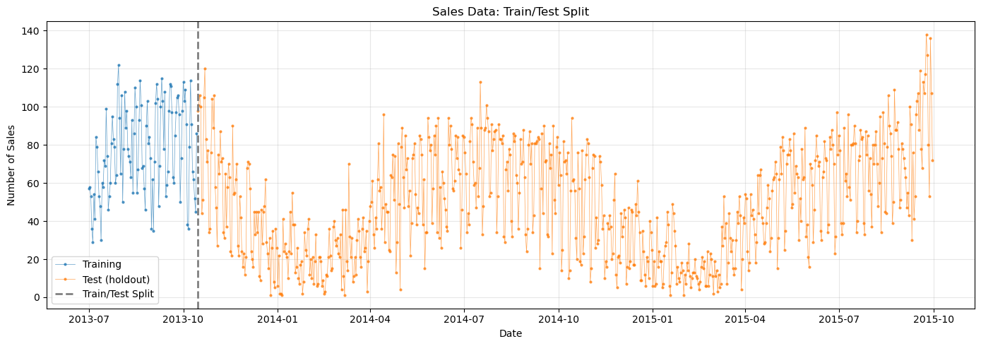
The challenge: We need to forecast through winter with only summer/fall data!
Baseline: Prophet-like Model Without Transfer Learning#
First, let’s see what happens when we fit a standard Prophet-like model to the short training data — with yearly seasonality but no prior knowledge about its shape.
This is what most practitioners would try first, and it’s exactly what fails in this scenario.
[7]:
# Baseline model: Prophet-like with uninformed yearly seasonality
baseline_model = (
    LinearTrend(n_changepoints=5)  # Linear trend with 5 changepoints seems to work best
    + FourierSeasonality(period=365.25, series_order=6)  # Yearly
    + FourierSeasonality(period=91.31, series_order=4)  # Quarterly
    + FourierSeasonality(period=30.44, series_order=3)  # Monthly
    + FourierSeasonality(period=7, series_order=2)  # Weekly
)

print("Fitting baseline model (no transfer learning)...")
baseline_model.fit(sales_train, method="mapx", scaler="minmax")

# Predict over the full date range (train + test)
baseline_pred = baseline_model.predict(horizon=len(sales_test), freq="D")
print("Done!")
Fitting baseline model (no transfer learning)...
WARNING:2026-02-27 00:19:23,619:jax._src.xla_bridge:876: An NVIDIA GPU may be present on this machine, but a CUDA-enabled jaxlib is not installed. Falling back to cpu.
Done!
[8]:
# Plot baseline predictions vs actual data
fig, ax = plt.subplots(figsize=(14, 6))

# Training data
ax.plot(
    sales_train["ds"],
    sales_train["y"],
    "C0o",
    markersize=3,
    alpha=0.5,
    label="Training data",
)

# Test data (ground truth)
ax.plot(
    sales_test["ds"],
    sales_test["y"],
    "C1o",
    markersize=3,
    alpha=0.5,
    label="Test data (actual)",
)

# Baseline prediction
ax.plot(
    baseline_pred["ds"],
    baseline_pred["yhat_0"],
    "C3-",
    linewidth=1.5,
    alpha=0.8,
    label="Baseline prediction",
)

ax.axvline(
    train_test_date, color="gray", linestyle="--", linewidth=2, label="Train/Test Split"
)
ax.set_title("Baseline Model: Prophet-like without Transfer Learning")
ax.set_xlabel("Date")
ax.set_ylabel("Number of Rides")
ax.legend(loc="upper right")
ax.grid(True, alpha=0.3)
plt.tight_layout()
plt.show()

print("\nObservation: The baseline model fails to capture yearly seasonality!")
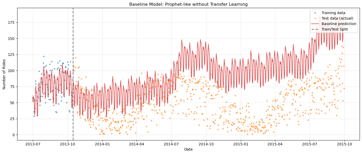
Observation: The baseline model fails to capture yearly seasonality!
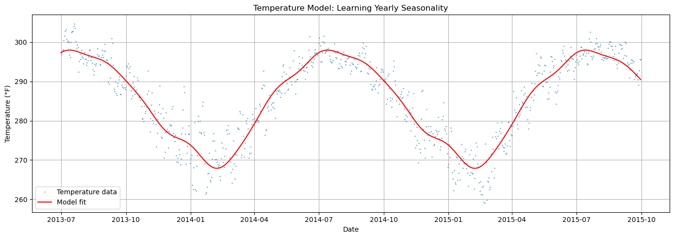
Step 1: Learn Seasonality from Temperature Data#
Now we fit a model to the long temperature time series. The goal is to learn the shape of yearly seasonality — specifically, the posterior distribution of the Fourier coefficients.
Since temperature is much simpler than sales (just yearly seasonality, no weekly pattern, minimal trend), we use a simple model.
[9]:
# Temperature model: Simple trend + yearly seasonality
# We use a very simple flat trend since we do not expect temperature to have growth
temp_model = FlatTrend() + FourierSeasonality(period=365.25, series_order=6)

print("Fitting temperature model to learn yearly seasonality...")
temp_model.fit(temp_df, method="nuts", scaler="minmax")

# Get predictions to visualize the fit
temp_pred = temp_model.predict(horizon=0, freq="D")
print("Done!")
Fitting temperature model to learn yearly seasonality...
Multiprocess sampling (4 chains in 4 jobs)
NUTS: [ft_0 - intercept, fs_0 - beta(p=365.25,n=6), sigma]
Sampling 4 chains for 1_000 tune and 1_000 draw iterations (4_000 + 4_000 draws total) took 8 seconds.
Done!
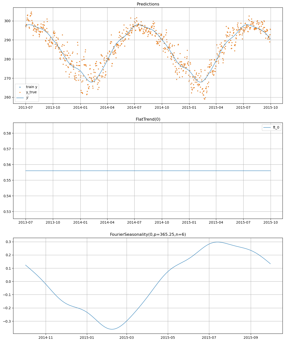
[10]:
# Visualize temperature model fit
fig, ax = plt.subplots(figsize=(14, 5))

ax.plot(temp_df["ds"], temp_df["y"], "C0.", markersize=1, label="Temperature data")
ax.plot(temp_pred["ds"], temp_pred["yhat_0"], "r-", linewidth=1.5, label="Model fit")

ax.set_title("Temperature Model: Learning Yearly Seasonality")
ax.set_xlabel("Date")
ax.set_ylabel("Temperature (°F)")
ax.legend()
ax.grid(True)
plt.tight_layout()
plt.show()
[11]:
# Plot the component decomposition for the temperature model
temp_model.plot(temp_pred, y_true=temp_df)
The Learned Fourier Coefficients#
The temperature model has learned 12 Fourier coefficients (6 sine + 6 cosine terms) that describe the yearly seasonal pattern. These coefficients, stored in trace, will be transferred as priors to the sales model.
Using the tune_method="parametric" option, vangja automatically extracts the posterior mean and standard deviation of these coefficients and uses them as the prior for the new model.
[12]:
# Inspect the learned Fourier coefficients from the temperature model
# These are stored in the trace attribute after fitting
beta_key = "fs_0 - beta(p=365.25,n=6)"
beta_posterior = temp_model.trace["posterior"][beta_key]

# Calculate mean and std (what parametric tuning will use)
beta_mean = beta_posterior.mean(dim=["chain", "draw"]).values
beta_std = beta_posterior.std(dim=["chain", "draw"]).values

print("Learned Fourier coefficients from temperature model:")
print("-" * 50)
for i in range(len(beta_mean)):
    term_type = "sin" if i % 2 == 0 else "cos"
    order = (i // 2) + 1
    print(
        f"  {term_type}(order={order}): mean = {beta_mean[i]:7.3f}, std = {beta_std[i]:.4f}"
    )

print("\nThese posteriors will become the priors for the sales model!")
Learned Fourier coefficients from temperature model:
--------------------------------------------------
  sin(order=1): mean =  -0.122, std = 0.0041
  cos(order=1): mean =  -0.280, std = 0.0042
  sin(order=2): mean =  -0.029, std = 0.0042
  cos(order=2): mean =  -0.001, std = 0.0043
  sin(order=3): mean =  -0.010, std = 0.0041
  cos(order=3): mean =   0.018, std = 0.0043
  sin(order=4): mean =   0.004, std = 0.0041
  cos(order=4): mean =   0.017, std = 0.0042
  sin(order=5): mean =  -0.002, std = 0.0042
  cos(order=5): mean =   0.002, std = 0.0042
  sin(order=6): mean =   0.000, std = 0.0041
  cos(order=6): mean =   0.009, std = 0.0041

These posteriors will become the priors for the sales model!
As in any transfer learning scenario, we also need to be careful to extract the scaling parameters for the timestamp column in temp_model.data. Let’s take a look at them.
[13]:
temp_model.t_scale_params
[13]:
{'ds_min': Timestamp('2013-07-01 00:00:00'),
 'ds_max': Timestamp('2015-09-30 00:00:00')}
Step 2: Transfer Learning to the Sales Model#
Now we create a new model for sales that:
Has its own trend and weekly seasonality (learned from sales data)
Transfers the yearly seasonality from the temperature model via
tune_method="parametric"
The tune_method="parametric" setting tells the FourierSeasonality component to:
Extract the posterior mean and std of the Fourier coefficients from
idataUse these as the prior mean and std for the new model’s coefficients
This gives the sales model a strong, informed prior about what yearly seasonality looks like — even though it has never seen a full year of sales data.
[14]:
# Transfer learning model: Use learned yearly seasonality
transfer_model = (
    FlatTrend()  # No trend, since we have very little data and don't want to overfit a trend
    + FourierSeasonality(
        period=365.25,
        series_order=6,
        tune_method="parametric",  # KEY: Transfer from temperature model
    )
    + FourierSeasonality(period=91.31, series_order=4)  # Quarterly (learned from sales)
    + FourierSeasonality(period=30.44, series_order=3)  # Monthly (learned from sales)
    + FourierSeasonality(period=7, series_order=3)  # Weekly (learned from sales)
)

print("Fitting transfer learning model...")
print("  - Flat trend: no trend learned from sales data")
print("  - Weekly seasonality: learned from sales data")
print("  - Monthly seasonality: learned from sales data")
print("  - Quarterly seasonality: learned from sales data")
print("  - Yearly seasonality: TRANSFERRED from temperature model")

# Pass the temperature model's trace and scaling parameters to transfer the learned seasonality
transfer_model.fit(
    sales_train,
    method="mapx",
    idata=temp_model.trace,
    t_scale_params=temp_model.t_scale_params,
    scaler="minmax",
)

# Predict over the full date range
transfer_pred = transfer_model.predict(horizon=len(sales_test), freq="D")

# Keep only the predictions for the train + test period (since predict returns the full range)
transfer_pred = transfer_pred[
    (transfer_pred["ds"] >= sales_train["ds"].min())
    & (transfer_pred["ds"] <= sales_test["ds"].max())
]
print("Done!")
Fitting transfer learning model...
  - Flat trend: no trend learned from sales data
  - Weekly seasonality: learned from sales data
  - Monthly seasonality: learned from sales data
  - Quarterly seasonality: learned from sales data
  - Yearly seasonality: TRANSFERRED from temperature model
Done!
[15]:
# Plot transfer learning predictions vs actual data
fig, ax = plt.subplots(figsize=(14, 6))

# Training data
ax.plot(
    sales_train["ds"],
    sales_train["y"],
    "C0o",
    markersize=3,
    alpha=0.5,
    label="Training data",
)

# Test data (ground truth)
ax.plot(
    sales_test["ds"],
    sales_test["y"],
    "C1o",
    markersize=3,
    alpha=0.5,
    label="Test data (actual)",
)

# Transfer learning prediction
ax.plot(
    transfer_pred["ds"],
    transfer_pred["yhat_0"],
    "C2-",
    linewidth=1.5,
    alpha=0.8,
    label="Transfer learning prediction",
)

ax.axvline(
    train_test_date, color="gray", linestyle="--", linewidth=2, label="Train/Test Split"
)
ax.set_title("Transfer Learning Model: Yearly Seasonality from Temperature")
ax.set_xlabel("Date")
ax.set_ylabel("Number of Sales")
ax.legend(loc="upper right")
ax.grid(True, alpha=0.3)
plt.tight_layout()
plt.show()

print("\nObservation: The transfer learning model captures the winter drop!")
print("It correctly predicts lower demand in winter and recovery in spring/summer.")
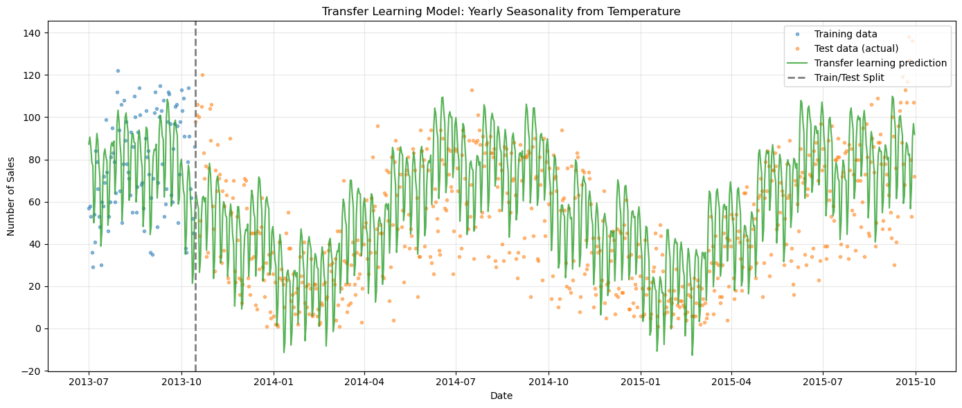
Observation: The transfer learning model captures the winter drop!
It correctly predicts lower demand in winter and recovery in spring/summer.
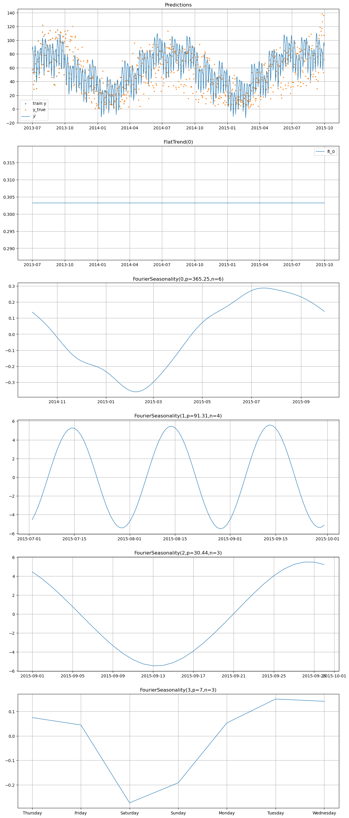
[16]:
# Plot component decomposition for the transfer learning model
transfer_model.plot(transfer_pred, y_true=sales_df)
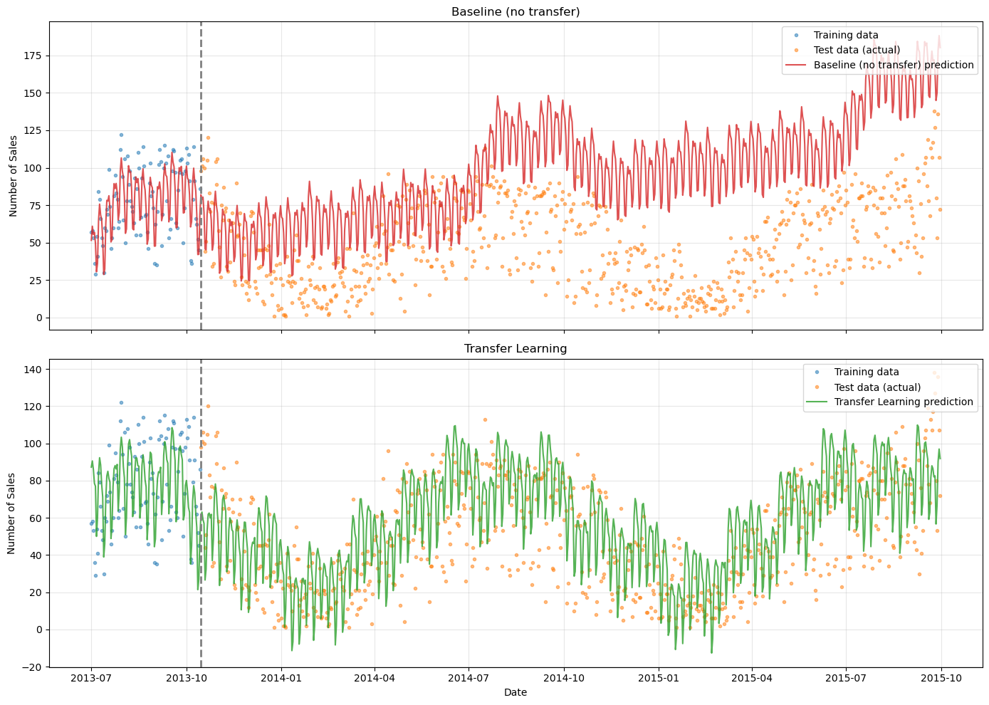
Comparison: Baseline vs Transfer Learning#
Let’s compare both models side-by-side to see the dramatic improvement from transfer learning.
[17]:
# Side-by-side comparison
fig, axes = plt.subplots(2, 1, figsize=(14, 10), sharex=True)

for ax, (model_name, pred, color) in zip(
    axes,
    [
        ("Baseline (no transfer)", baseline_pred, "C3"),
        ("Transfer Learning", transfer_pred, "C2"),
    ],
):
    # Training data
    ax.plot(
        sales_train["ds"],
        sales_train["y"],
        "C0o",
        markersize=3,
        alpha=0.5,
        label="Training data",
    )

    # Test data (ground truth)
    ax.plot(
        sales_test["ds"],
        sales_test["y"],
        "C1o",
        markersize=3,
        alpha=0.5,
        label="Test data (actual)",
    )

    # Model prediction
    ax.plot(
        pred["ds"],
        pred["yhat_0"],
        f"{color}-",
        linewidth=1.5,
        alpha=0.8,
        label=f"{model_name} prediction",
    )

    ax.axvline(train_test_date, color="gray", linestyle="--", linewidth=2)
    ax.set_title(f"{model_name}")
    ax.set_ylabel("Number of Sales")
    ax.legend(loc="upper right")
    ax.grid(True, alpha=0.3)

axes[-1].set_xlabel("Date")
plt.tight_layout()
plt.show()
[18]:
# Overlay comparison
fig, ax = plt.subplots(figsize=(14, 6))

# Training data
ax.plot(
    sales_train["ds"],
    sales_train["y"],
    "C0o",
    markersize=3,
    alpha=0.4,
    label="Training data",
)

# Test data (ground truth)
ax.plot(
    sales_test["ds"],
    sales_test["y"],
    "C1o",
    markersize=3,
    alpha=0.4,
    label="Test data (actual)",
)

# Both predictions
ax.plot(
    baseline_pred["ds"],
    baseline_pred["yhat_0"],
    "C3-",
    linewidth=1.5,
    alpha=0.8,
    label="Baseline prediction",
)
ax.plot(
    transfer_pred["ds"],
    transfer_pred["yhat_0"],
    "C2-",
    linewidth=1.5,
    alpha=0.8,
    label="Transfer learning prediction",
)

ax.axvline(
    train_test_date, color="gray", linestyle="--", linewidth=2, label="Train/Test Split"
)
ax.set_title("Comparison: Baseline vs Transfer Learning")
ax.set_xlabel("Date")
ax.set_ylabel("Number of Sales")
ax.legend(loc="upper right")
ax.grid(True, alpha=0.3)
plt.tight_layout()
plt.show()
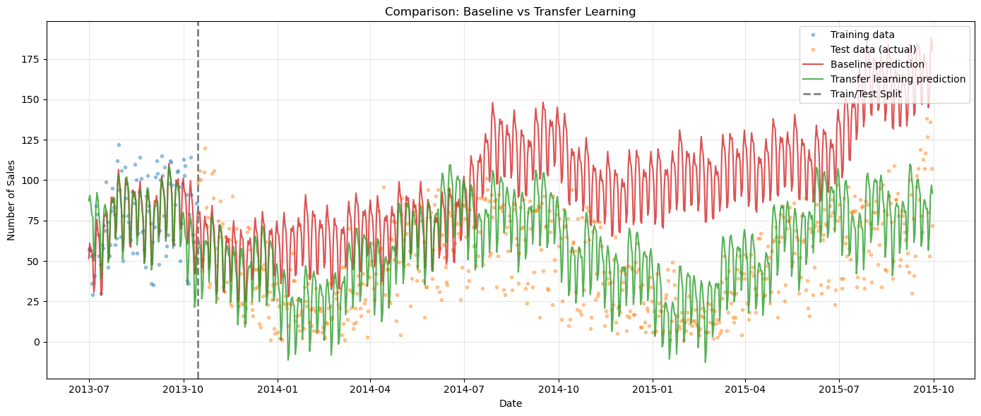
Quantitative Comparison#
Let’s compute error metrics on the test set to quantify the improvement.
[19]:
# Calculate metrics
baseline_metrics = metrics(sales_test, baseline_pred, pool_type="complete")
transfer_metrics = metrics(sales_test, transfer_pred, pool_type="complete")

# Also compute a simple mean baseline
mean_pred_value = sales_train["y"].mean()
mean_metrics = pd.DataFrame(
    {
        "mse": {"series": np.mean((sales_test["y"].values - mean_pred_value) ** 2)},
        "rmse": {
            "series": np.sqrt(np.mean((sales_test["y"].values - mean_pred_value) ** 2))
        },
        "mae": {"series": np.mean(np.abs(sales_test["y"].values - mean_pred_value))},
        "mape": {
            "series": np.mean(
                np.abs(
                    (sales_test["y"].values - mean_pred_value) / sales_test["y"].values
                )
            )
            * 100
        },
    },
    index=["series"],
)

# Display comparison table
comparison_df = pd.DataFrame(
    {
        "Mean Baseline": mean_metrics.iloc[0],
        "Prophet-like (no transfer)": baseline_metrics.iloc[0],
        "Transfer Learning": transfer_metrics.iloc[0],
    },
).T

print("Test Set Metrics Comparison")
print("=" * 60)
display(comparison_df.round(2))
Test Set Metrics Comparison
============================================================
| mse | rmse | mae | mape | |
|---|---|---|---|---|
| Mean Baseline | 1639.94 | 40.50 | 33.71 | 265.54 |
| Prophet-like (no transfer) | 3563.91 | 59.70 | 52.58 | 2.86 |
| Transfer Learning | 472.67 | 21.74 | 17.34 | 0.90 |
[20]:
# Calculate improvement percentages
rmse_improvement = (1 - transfer_metrics["rmse"] / baseline_metrics["rmse"]) * 100
mae_improvement = (1 - transfer_metrics["mae"] / baseline_metrics["mae"]) * 100

print("\nImprovement from Transfer Learning:")
print(f"  RMSE reduction: {rmse_improvement.values[0]:.1f}%")
print(f"  MAE reduction:  {mae_improvement.values[0]:.1f}%")
Improvement from Transfer Learning:
  RMSE reduction: 63.6%
  MAE reduction:  67.0%
How It Works: The Parametric Transfer#
The tune_method="parametric" option in vangja implements a simple but powerful form of Bayesian transfer learning:
Step 1: Fit the Source Model#
You fit the temperature model to the long time series using MCMC sampling or Variational Inference (Maximum A Posteriori estimates do not produce posterior uncertainty). For example:
temp_model.fit(temp_df, method="nuts")
The temperature model learns Fourier coefficients \(\beta_1, \ldots, \beta_{12}\) from ~5 years of data. The posterior is stored in temp_model.idata_.
Step 2: Extract Posterior Statistics#
When fitting the sales model with idata=temp_model.trace, vangja extracts:
\(\mu_i = \mathbb{E}[\beta_i | \text{data}]\) — posterior mean
\(\sigma_i = \text{Std}[\beta_i | \text{data}]\) — posterior standard deviation
You can manually extract the posterior samples and compute different statistics if you want. Vangja allows you to pass these directly as override_... parameters in every component. Read the API docs for details.
Step 3: Set Informed Priors#
The sales model’s Fourier coefficients receive Normal priors:
This is much more informative than the default \(\beta \sim \text{Normal}(0, 10)\). The sales model’s optimization process now starts with a strong belief about the seasonal shape, learned from temperature.
Why This Works#
Temperature and bike sales share a causal driver: weather/seasons. When temperature drops in winter:
Fewer people want to bike in the cold
The yearly seasonal pattern in temperature correlates with bike demand
By learning the shape of yearly seasonality from temperature (where we have years of data), we can transfer this knowledge to sales (where we have only months).
Limitations and Considerations#
What We Simplified#
The original blog posts use a more sophisticated model:
Negative binomial likelihood for count data (we use Gaussian)
Autoregressive dynamics: \(\mu_t = (1-\delta-\eta)\lambda_t + \delta\mu_{t-1} + \eta y_{t-1}\)
Day-of-week effects as explicit dummy variables
Vangja’s approach is simpler:
We use a Gaussian likelihood (adequate for this scale of data)
Instead of AR dynamics, we use
LinearTrendwith changepointsWeekly seasonality is learned via
FourierSeasonality(period=7)We add a monthly and quarterly Fourier seasonality to capture additional patterns
Despite these simplifications, the core insight — transferring learned seasonality via Bayesian priors — works well.
When Transfer Learning Helps#
Transfer learning is most valuable when:
Short target series: Not enough data to learn long-term patterns
Long source series: Available related data with the pattern you need
Shared patterns: The source and target genuinely share the pattern to transfer
Potential Pitfalls#
Over-confident priors: If the temperature seasonality doesn’t match sales at all, strong priors could hurt. Consider overriding the
beta_sdparameter for tuning or using less restrictive priors.Scale mismatch: Temperature is in °F, sales is in counts. Vangja handles this by scaling data internally, and the Fourier coefficients represent shape, not magnitude.
Phase mismatch: If the seasonal peaks don’t align (e.g., sales peak occurs 2 weeks after temperature peak), you may need the
shift_for_tuneoption. Look at the API docs for details on how to use it.
Summary#
In this chapter, we demonstrated how to use transfer learning to forecast short time series with vangja:
The Problem: With only ~3 months of bike sales data, standard methods fail to capture yearly seasonality, leading to wildly optimistic winter forecasts.
The Solution: Learn yearly seasonality from a related long time series (NYC temperature, ~5 years) and transfer it as informed priors to the sales model.
The Implementation:
Fit a model to temperature data to learn Fourier coefficients
Create a sales model with
tune_method="parametric"on yearly seasonalityPass
idata=temp_model.idata_to transfer the learned posteriors as priors
The Result: The transfer learning model captures the winter demand drop and achieves significantly lower forecast errors than the baseline.
Key Takeaways#
Transfer learning in vangja uses
tune_method="parametric"to pass posterior mean/std as new priorsFind a proxy: When your target series is short, look for a longer related series that shares patterns
Domain knowledge matters: The insight that temperature correlates with bike demand made this transfer work
Simple can work: Even with Vangja’s simpler Prophet-like approach (vs. the original AR model), the core transfer learning insight delivers strong results
Further Reading#
Modeling Short Time Series with Prior Knowledge — the original blog post by Tim Radtke
Modeling Short Time Series with Prior Knowledge in PyMC — Juan Orduz’s PyMC implementation
Rob Hyndman: Fitting Models to Short Time Series — context on the challenges of short series forecasting
What’s Next#
In Chapter 08, we explore a more powerful transfer learning method — tune_method="prior_from_idata" — which preserves the full posterior covariance structure. We also show how to combine hierarchical modeling with transfer learning in a single model, leveraging the strengths of both approaches.