Chapter 02: Inference Algorithms

This notebook explores the different Bayesian inference algorithms available in vangja. We’ll use the multiplicative model from the Air Passengers dataset to compare:

1. Maximum A Posteriori (MAP) — Point estimates

2. Variational Inference (ADVI) — Approximate posterior

3. Markov Chain Monte Carlo (NUTS) — Full posterior sampling

Each method offers different trade-offs between computational speed and the richness of uncertainty quantification.

Reference: For a detailed exploration of these Bayesian inference techniques in time series forecasting, see Krajevski & Tojtovska Ribarski (2026): Going NUTS with ADVI: Exploring various Bayesian Inference techniques with Facebook Prophet, arXiv:2601.20120.

Setup and Imports

import warnings

warnings.filterwarnings("ignore")

import time

import matplotlib.pyplot as plt
import numpy as np
import pandas as pd

from vangja import FourierSeasonality, LinearTrend
from vangja.datasets import load_air_passengers
from vangja.utils import metrics

# Set random seed for reproducibility
np.random.seed(42)

print("Imports successful!")

Imports successful!

Load and Prepare Data

We’ll use the same Air Passengers dataset from the Getting Started notebook.

# Load Air Passengers dataset from vangja.datasets
air_passengers = load_air_passengers()

# Split data: use last 12 months for testing
train = air_passengers[:-12].copy()
test = air_passengers[-12:].copy()

print(
    f"Training set: {train['ds'].min()} to {train['ds'].max()} ({len(train)} samples)"
)
print(f"Test set: {test['ds'].min()} to {test['ds'].max()} ({len(test)} samples)")

Training set: 1949-01-01 00:00:00 to 1959-12-01 00:00:00 (132 samples)
Test set: 1960-01-01 00:00:00 to 1960-12-01 00:00:00 (12 samples)

Define the Multiplicative Model

We’ll use a multiplicative model that captures the increasing variance with trend:

\[y(t) = g(t) \cdot (1 + s(t)) + \epsilon\]

where \(g(t)\) is the linear trend and \(s(t)\) is the combined seasonality.

def create_model():
    """Create a fresh multiplicative model instance."""
    return LinearTrend(n_changepoints=25) ** (
        FourierSeasonality(period=365.25, series_order=10)
        + FourierSeasonality(period=7, series_order=3)
    )


print(f"Model structure: {create_model()}")

Model structure: LT(n=25,r=0.8,tm=None) * (1 + FS(p=365.25,n=10,tm=None) + FS(p=7,n=3,tm=None))

---

1. Maximum A Posteriori (MAP) Estimation

What is MAP?

Maximum A Posteriori (MAP) estimation finds the single most probable parameter values given the data and priors. Mathematically, MAP finds:

\[\hat{\theta}_{MAP} = \arg\max_{\theta} P(\theta | D) = \arg\max_{\theta} P(D | \theta) \cdot P(\theta)\]

where \(P(D | \theta)\) is the likelihood and \(P(\theta)\) is the prior.

Advantages:

• Very fast computation

• Good for quick prototyping and model comparison

• Works well when you have enough data

Limitations:

• Provides only a point estimate (no uncertainty quantification)

• Can get stuck in local optima

• Doesn’t capture the full shape of the posterior distribution

PyMC’s map vs pymc-extras’ mapx

Vangja supports two MAP implementations:

Feature	map (PyMC)	mapx (pymc-extras)
Backend	SciPy optimizers	JAX-based optimization
Speed	Slower	Significantly faster
Gradient computation	Numerical or PyTensor	JAX autodiff
Recommended	Legacy support	Default choice

The mapx method from pymc-extras uses JAX for automatic differentiation, resulting in much faster optimization, especially for models with many parameters.

1.1 MAP with mapx (Recommended)

# Create and fit the model using mapx (default)
model_mapx = create_model()

start_time = time.time()
model_mapx.fit(train, method="mapx")
mapx_time = time.time() - start_time

print(f"MAPX fitting time: {mapx_time:.2f} seconds")

WARNING:2026-02-26 20:45:49,639:jax._src.xla_bridge:876: An NVIDIA GPU may be present on this machine, but a CUDA-enabled jaxlib is not installed. Falling back to cpu.

MAPX fitting time: 8.82 seconds

# Predict and evaluate
future_mapx = model_mapx.predict(horizon=365, freq="D")
metrics_mapx = metrics(test, future_mapx, "complete")

print("MAPX Metrics:")
display(metrics_mapx)

MAPX Metrics:

	mse	rmse	mae	mape
series	629.010786	25.080087	21.254398	0.04267

1.2 MAP with map (Standard PyMC)

# Create and fit the model using standard PyMC map
model_map = create_model()

start_time = time.time()
model_map.fit(train, method="map")
map_time = time.time() - start_time

print(f"MAP fitting time: {map_time:.2f} seconds")
print(f"Speedup with mapx: {map_time / mapx_time:.1f}x faster")

MAP fitting time: 6.71 seconds
Speedup with mapx: 0.8x faster

# Predict and evaluate
future_map = model_map.predict(horizon=365, freq="D")
metrics_map = metrics(test, future_map, "complete")

print("MAP Metrics:")
display(metrics_map)

MAP Metrics:

	mse	rmse	mae	mape
series	648.633502	25.468284	21.179644	0.042348

---

2. Variational Inference (ADVI)

What is Variational Inference?

Variational Inference (VI) approximates the true posterior distribution \(P(\theta | D)\) with a simpler distribution \(Q(\theta)\) from a tractable family. The goal is to minimize the Kullback-Leibler (KL) divergence between \(Q\) and the true posterior:

\[Q^* = \arg\min_Q KL(Q(\theta) || P(\theta | D))\]

Automatic Differentiation Variational Inference (ADVI)

ADVI is a specific VI algorithm that:

1. Transforms all parameters to unconstrained space

2. Approximates the posterior with a multivariate Gaussian

3. Uses gradient-based optimization to find the best approximation

Advantages:

• Much faster than MCMC

• Provides uncertainty estimates (unlike MAP)

• Scales well to large datasets

Limitations:

• Approximation may miss multimodal posteriors

• Gaussian assumption may be too restrictive

• Can underestimate uncertainty

Variants

Method	Description
advi	Mean-field approximation (diagonal covariance)
fullrank_advi	Full covariance matrix (captures correlations)

# Create and fit the model using ADVI
model_advi = create_model()

start_time = time.time()
model_advi.fit(
    train,
    method="advi",
    n=50000,  # number of ADVI iterations
    samples=1000,  # number of posterior samples to draw after ADVI convergence
)
advi_time = time.time() - start_time

print(f"ADVI fitting time: {advi_time:.2f} seconds")

Finished [100%]: Average Loss = -7.8993

ADVI fitting time: 37.00 seconds

# Predict and evaluate
future_advi = model_advi.predict(horizon=365, freq="D")
metrics_advi = metrics(test, future_advi, "complete")

print("ADVI Metrics:")
display(metrics_advi)

ADVI Metrics:

	mse	rmse	mae	mape
series	490.516804	22.147614	19.328256	0.040094

---

3. Markov Chain Monte Carlo (NUTS)

What is MCMC?

Markov Chain Monte Carlo (MCMC) methods generate samples from the posterior distribution by constructing a Markov chain that has the posterior as its stationary distribution. After enough iterations, the samples approximate the true posterior.

No-U-Turn Sampler (NUTS)

NUTS is an advanced MCMC algorithm that:

1. Uses Hamiltonian dynamics to propose distant moves

2. Automatically tunes the trajectory length (no manual tuning needed)

3. Avoids random walk behavior, leading to efficient exploration

Advantages:

• Provides the gold standard for posterior inference

• Captures the full posterior distribution, including multimodality

• Accurate uncertainty quantification

• Diagnostic tools available (R-hat, ESS, divergences)

Limitations:

• Computationally expensive

• Requires tuning (warmup/burn-in period)

• May have convergence issues for complex models

Sampler Backends

Vangja supports multiple NUTS backends:

Backend	Description
pymc	Default PyMC sampler
nutpie	Fast Rust-based sampler
numpyro	JAX-based sampler (GPU support)
blackjax	JAX-based sampler

# Create and fit the model using NUTS
# Using fewer samples for demonstration (increase for production)
model_nuts = create_model()

start_time = time.time()
model_nuts.fit(
    train,
    method="nuts",
    samples=1000,  # Number of posterior samples per chain
    chains=4,  # Number of independent chains
    cores=4,  # Parallel cores to use
)
nuts_time = time.time() - start_time

print(f"NUTS fitting time: {nuts_time:.2f} seconds")

Multiprocess sampling (4 chains in 4 jobs)
NUTS: [lt_0 - slope, lt_0 - intercept, lt_0 - delta, fs_0 - beta(p=365.25,n=10), fs_1 - beta(p=7,n=3), sigma]

Sampling 4 chains for 1_000 tune and 1_000 draw iterations (4_000 + 4_000 draws total) took 227 seconds.

NUTS fitting time: 230.79 seconds

# Predict and evaluate
future_nuts = model_nuts.predict(horizon=365, freq="D")
metrics_nuts = metrics(test, future_nuts, "complete")

print("NUTS Metrics:")
display(metrics_nuts)

NUTS Metrics:

	mse	rmse	mae	mape
series	698.054001	26.420712	22.329609	0.044714

---

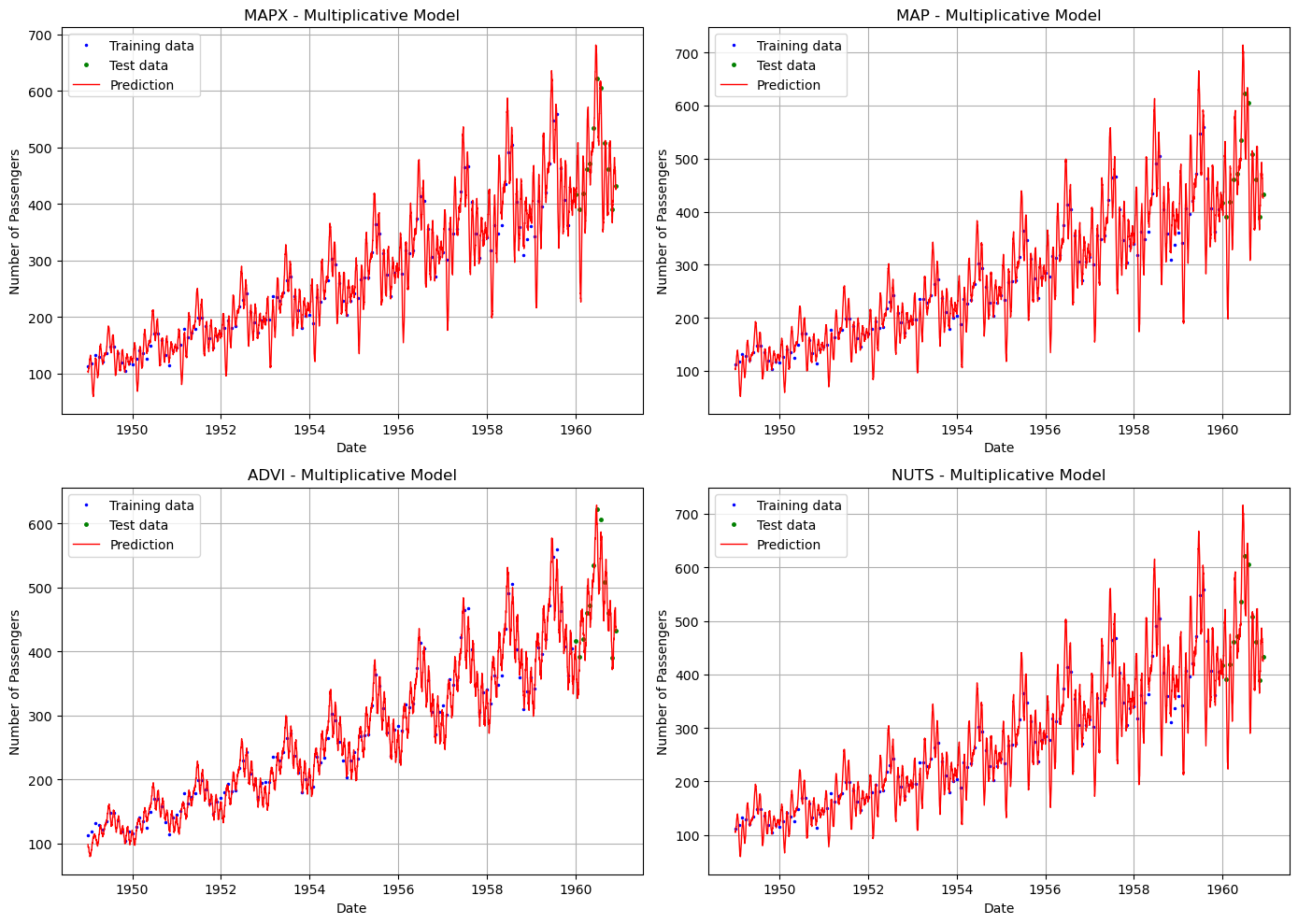
Comparison of Results

Let’s compare all inference methods side by side.

# Combine all metrics
comparison = pd.DataFrame(
    {
        "Method": ["MAPX", "MAP", "ADVI", "NUTS"],
        "Time (s)": [mapx_time, map_time, advi_time, nuts_time],
        "RMSE": [
            metrics_mapx["rmse"].values[0],
            metrics_map["rmse"].values[0],
            metrics_advi["rmse"].values[0],
            metrics_nuts["rmse"].values[0],
        ],
        "MAE": [
            metrics_mapx["mae"].values[0],
            metrics_map["mae"].values[0],
            metrics_advi["mae"].values[0],
            metrics_nuts["mae"].values[0],
        ],
        "MAPE": [
            metrics_mapx["mape"].values[0],
            metrics_map["mape"].values[0],
            metrics_advi["mape"].values[0],
            metrics_nuts["mape"].values[0],
        ],
    }
)

print("\nComparison of Inference Methods:")
display(comparison)

Comparison of Inference Methods:

	Method	Time (s)	RMSE	MAE	MAPE
0	MAPX	8.824514	25.080087	21.254398	0.042670
1	MAP	6.714782	25.468284	21.179644	0.042348
2	ADVI	37.004420	22.147614	19.328256	0.040094
3	NUTS	230.786814	26.420712	22.329609	0.044714

# Visual comparison of predictions
fig, axes = plt.subplots(2, 2, figsize=(14, 10))

methods = [
    ("MAPX", future_mapx),
    ("MAP", future_map),
    ("ADVI", future_advi),
    ("NUTS", future_nuts),
]

for ax, (name, future) in zip(axes.flat, methods):
    ax.plot(train["ds"], train["y"], "b.", label="Training data", markersize=3)
    ax.plot(test["ds"], test["y"], "g.", label="Test data", markersize=5)
    ax.plot(future["ds"], future["yhat_0"], "r-", label="Prediction", linewidth=1)
    ax.set_title(f"{name} - Multiplicative Model")
    ax.set_xlabel("Date")
    ax.set_ylabel("Number of Passengers")
    ax.legend()
    ax.grid(True)

plt.tight_layout()
plt.show()

---

Summary: Choosing an Inference Method

Method	Speed	Uncertainty	Best For
MAPX	⚡⚡⚡ Fastest	❌ None	Quick prototyping, model selection, production with large data
MAP	⚡⚡ Fast	❌ None	Legacy compatibility
ADVI	⚡⚡ Fast	✅ Approximate	When you need uncertainty but MCMC is too slow
NUTS	⚡ Slow	✅✅ Full	Research, when accuracy matters most, small to medium data

Transfer Learning Consideration

When using vangja’s transfer learning capabilities (fitting short time series with priors from long time series), MCMC methods are particularly valuable because:

• They capture the full posterior from the long time series

• The posterior can be used directly as a prior for the short series

• Uncertainty propagates correctly through the transfer process

What’s Next

In Chapter 03, we explore vangja’s ability to fit multiple time series simultaneously using vectorized computations — a significant performance advantage over fitting each series one at a time.